Purpose
We’re interested in using spontaneous Raman spectroscopy as a readout for the chemical state of biological systems. Previous efforts have reported that Raman spectroscopy can be used to distinguish between different strains 1, cell types 2, and physiological states 3–4. In an effort to obtain analogous results relevant to our own work, we acquired spontaneous spectra of two small collections of yeast strains, then trained conventional machine learning models to predict both strain and species identity from the Raman spectra alone. We found that, in this dataset, experimental batch effects dominated strain-level biological signals but not species-level signals. As similar batch effects may be present in other studies, careful experimental design is warranted, especially when machine learning is used for analysis.
This work is primarily for researchers using Raman spectroscopy to detect meaningful differences between biological variables of interest (e.g., species, strain, growth condition, cell type, cell state, etc). We're sharing these results to call attention to the existence of experimental batch effects in spontaneous Raman spectra of biological samples, and of the consequent importance of rigorous experimental design and cross-validated analysis when using this technique.
Background and goals
Raman spectroscopy offers a promising approach for distinguishing between biological samples, as it's label-free, requires minimal sample preparation, and may detect subtle chemical-compositional differences 5–6. Commonly, it's used as an initial screening step to identify samples or conditions of potential interest in a fast, non-destructive way, as a complement to rather than a replacement for high-resolution analytical methods 7–9. More recently, an alternative analytical framework has emerged that treats Raman spectra as feature vectors and trains machine learning models to predict biological labels of interest (such as sample identity, cell identity, or cell state) directly from held-out spectra 1–2, 10–12, potentially expanding the range of applications. Our goal here was to explore the utility of such data-driven approaches by evaluating whether Raman spectra can be used to distinguish between different strains and species of yeast and to understand the extent to which batch effects from experimental variation confound these predictions.
The approach
Experimental design
We collected Raman spectra from nine yeast strains, including wild-type and mutant strains from both Saccharomyces cerevisiae and Schizosaccharomyces pombe (Table 1). We generated three "end-to-end" biological replicates by repeating the sample preparation and imaging protocols in triplicate, each with separate cell cultures, physical plates, and imaging dates.
Species and strains
We chose to work with several strains of budding and fission yeast (Saccharomyces cerevisiae and Schizosaccharomyces pombe, respectively). Our dataset included three standard lab strains (BY4741, SP286, and ED666) along with six knockout strains (see Table 1) that were of interest to us because they encode orthologs of human proteins involved in disease.
| Species | Strain or gene ID | Genotype | Description | Source |
|---|---|---|---|---|
| S. cerevisiae | BY4741 | Standard haploid lab strain | ATCC | |
| S. cerevisiae | YGL058w | rad6Δ | Null mutant of rad6, an ortholog of human UBE2A (a ubiquitin-conjugating enzyme) | EUROSCARF |
| S. cerevisiae | YNL141w | aah1Δ | Null mutant of aah1, an ortholog of human ADA (an adenosine deaminase) | EUROSCARF |
| S. pombe | SP286 | Standard diploid lab strain | Bioneer | |
| S. pombe | ED666 | Standard haploid lab strain | Bioneer | |
| S. pombe | SPAC18B11.07c | rhp6Δ | Null mutant of rhp6, an ortholog of human UBE2A | Bioneer |
| S. pombe | SPBC1198.02 | dea2Δ/+ | Heterozygous null mutant of dea2 (an ortholog of human ADA) | Bioneer |
| S. pombe | SPBPB10D8.02c | asgΔ | Null mutant of asg (an ortholog of human ARSG, a lysosomal sulfatase) | Bioneer |
| S. pombe | SPBC530.12c | pdf1Δ/+ | Heterozygous null mutant of pdf1 (an ortholog of human PPT1, a lysosomal hydrolase) | Bioneer |
Table 1. List of species and strains used in this study.
The three standard lab strains are identified by their strain IDs, while the six mutant strains are identified by their gene IDs. The two heterozygous mutant strains are homozygous lethal. To find the strains from Bioneer, use the link provided and search the strain/gene ID in the “Search keyword” field.
Sample preparation and Raman spectroscopy
We inoculated each strain in 5 mL of rich media in a 15 mL culture tube. We grew S. cerevisiae strains in YPD media and grew the S. pombe strains in YES media. We grew cultures overnight in a shaking incubator (Infors HT) set to 30 °C, shaking at 200 rpm. We measured the OD600 for each strain using a spectrophotometer (Thermo Fisher Scientific, NanoDrop One/OneC). We diluted all strains to an OD600 of five in a final volume of 1 mL. We pelleted cells in 1.5 mL microcentrifuge tubes using a tabletop centrifuge (Thermo Scientific, Sorvall Legend Micro 21) at 3,000 × g for 3 min. We removed the supernatant and washed cells by resuspending in 1 mL of 0.9% saline solution. We pelleted cells again under the same conditions and removed the supernatant. We then washed cells by resuspending in 1 mL of deionized water, pelleting, and removing the supernatant. We spotted wet cell pellets onto stainless steel plates (stamped with a 96-well plate layout) and allowed them to desiccate at room temperature and pressure for approximately 3 h.
We acquired spontaneous Raman spectra of the desiccated samples using a probe-based Raman spectrometer with a 785 nm excitation (model WP-785X-F13-R-IL, Wasatch Photonics). We integrated the spectrometer with a motorized XY stage and controlled the hardware using Pycro-Manager 13 and custom Python scripts to enable fully automated acquisitions. We acquired spectra at a 5 × 5 grid of positions in each “well” on each of the three replicate plates, resulting in a total of 75 spectra for each strain. We acquired spectra with a laser power of 93 mW (measured at the sample plane), an integration time of five seconds, and 10 averages per position.
Data processing
The raw Raman spectra were processed using a standard pipeline based on the ramanspy Python package 14.
- Cosmic ray removal. We applied the Whitaker–Hayes despiking algorithm with default parameters to remove cosmic ray artifacts.
- Background subtraction. For each plate (i.e., for each experimental replicate), we acquired a dark spectrum from an empty region of the stainless steel plate. We computed a "consensus" background spectrum by averaging the dark spectra from all three plates, then subtracted this same consensus background spectrum from all sample spectra in the dataset. The use of a single background spectrum (rather than one per plate) is necessary to avoid injecting additional batch effects into the spectra from small per-plate differences in the background spectra.
- Quality control to remove low-intensity spectra. The unnormalized intensity of some spectra was too low to yield detectable Raman peaks. These spectra likely corresponded to regions of the well without sufficient desiccated material. We identified and removed these spectra by applying an empirically determined threshold of 1,000 intensity units to the mean intensity of the background-subtracted but otherwise unprocessed spectra.
- Smoothing and baseline correction. After background subtraction, we applied a Savitzky-Golay filter to smooth the spectra, then subtracted the autofluorescence background using the ModPoly algorithm with a polynomial order of five.
- Cropping and normalization. After baseline correction, we cropped the spectra to the "fingerprint region" (300–1,800 cm−1) and normalized the cropped spectra using area-under-the-curve (AUC) normalization.
- Quality control to remove outlier spectra. Within each well of each plate, we identified outlier spectra by computing the standard deviation of each spectrum's difference from the group median spectrum, then used elbow detection on the sorted distances to identify outliers. This quality control removed spectra that likely resulted from heterogeneous desiccation or imaging artifacts.
- Batch correction. To correct for plate-level batch effects, we used two independent approaches. In the first approach, we applied a linear mixed model to each wavenumber independently, treating plate identity as a random effect. We then corrected for plate-specific scale factors by normalizing the residuals by their within-batch standard deviations. This approach assumes that all batches are sufficiently large and that the random effect (plate identity) isn't confounded with the biological variable of interest (strain identity). In the second approach, we used an established third-party method, ComBat 15–16, with plate identity as the batch variable and no fixed effects. Note that, because all strains were present on all plates, we didn't need to include strain identity as a fixed effect in either model.
Analysis strategy
We treated each processed spectrum as a feature vector and the collection of all spectra as a feature matrix in which rows correspond to samples and columns to wavenumbers. We trained classifiers to predict strain identity and evaluated performance using two different cross-validation strategies:
- Standard k-fold cross-validation in which all spectra are randomly partitioned into training and test sets. This is the standard approach to cross-validation, and is often used in the literature for datasets that are known or assumed to be homogeneous and well-balanced.
- Leave-one-plate-out cross-validation in which spectra are partitioned into training and test sets according to the plate from which they came. This cross-validation strategy explicitly controls for experimental batch effects, as each of our three physical plates corresponds to an end-to-end experimental replicate.
After the QC steps described above, we were left with 24–33 spectra per strain (median 27). These spectra were distributed roughly evenly across the three physical plates. Because of these small sample sizes, we chose to use two conventional nonlinear classification models: a random forest and a support vector machine with an RBF kernel. We used the standard implementations from scikit-learn 17, with class weighting set to "balanced" to correct for class imbalances (which were minor, given our balanced experimental design). In the random forest model, we used 300 trees, and in the SVM, we used a value of 100 for the regularization parameter C. These values were chosen empirically. All other hyperparameters were set to their default values.
To evaluate classification performance, we plotted confusion matrices with counts normalized by the number of true members in each class. For a single overall performance metric, we also calculated the multiclass version of the Matthews correlation coefficient (MCC) as implemented in scikit-learn 17. This is a bounded metric in [−1, +1] that considers all elements of the confusion matrix and is therefore robust to class imbalances. A value of +1 corresponds to perfect predictions, a value of zero corresponds to random guessing, and a negative value indicates systemic misclassification. We computed this metric for the test set from each cross-validation fold, then computed the median across folds.
All code and data are available in our GitHub repo (DOI: 10.5281/zenodo.19226627).
Additional methods
We used Claude (Opus 4, 4.5, and 4.6) to help write, clean up, comment, and review our code, and we selectively incorporated its feedback. We also used Claude to suggest wording ideas and then chose which small phrases or sentence structure ideas to use, rearrange text to fit the structure of one of our pub templates, expand on summary text that we provided, and help clarify and streamline text that we wrote. Additionally, we chatted with Claude throughout the project to support ideation and analysis. We used Gemini (2.5 Pro) to review the publication to catch typos and discrepancies, and Cursor for tab completion while editing code.
We used arcadia-pycolor (v0.6.4) 18 to generate figures before manual adjustment.
The results
After processing, we found that the spectra contained a few clear, sharp peaks and many broad, diffuse features. In general, the mean spectra for all strains and species looked similar (Figure 1). We therefore reasoned that carefully cross-validated modeling (rather than exploratory analysis) would be necessary to determine whether the spectra contained genuine biological signals.
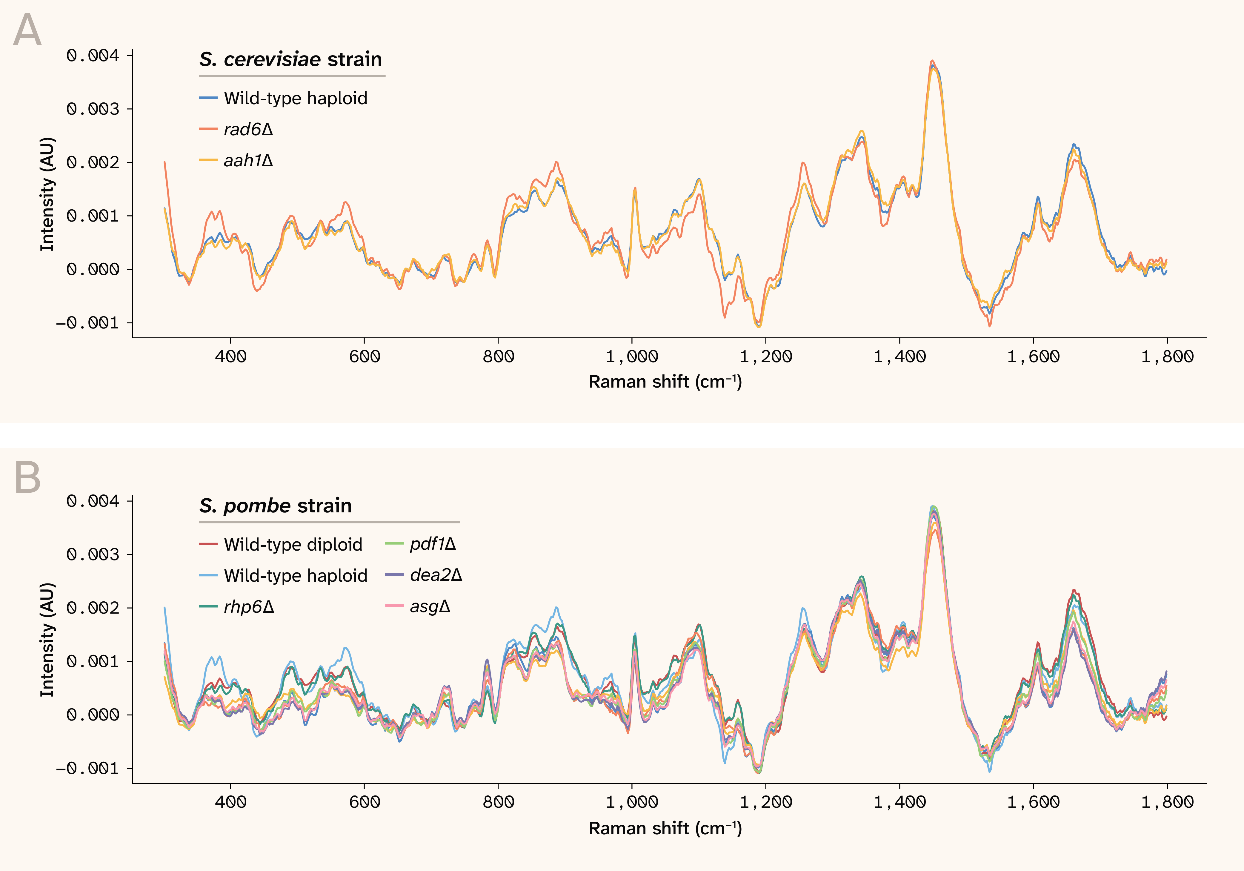
Figure 1. The overall mean spectra for each strain, grouped by species.
The spectra are baseline-subtracted and normalized. Note that the spectra can be negative due to fluctuations of the raw spectrum around the fitted baseline. AU: Arbitrary units.
Standard cross-validation gives misleadingly strong results
We first evaluated a strain classification task under standard k-fold cross-validation using five folds. The model performed well, with a median MCC of 0.79 (range 0.71–0.93). The confusion matrix showed a strong diagonal (Figure 2), indicating that the model correctly predicted strain identity across most samples. However, as we discuss below, the strain identities are confounded with plate identities in this analysis.
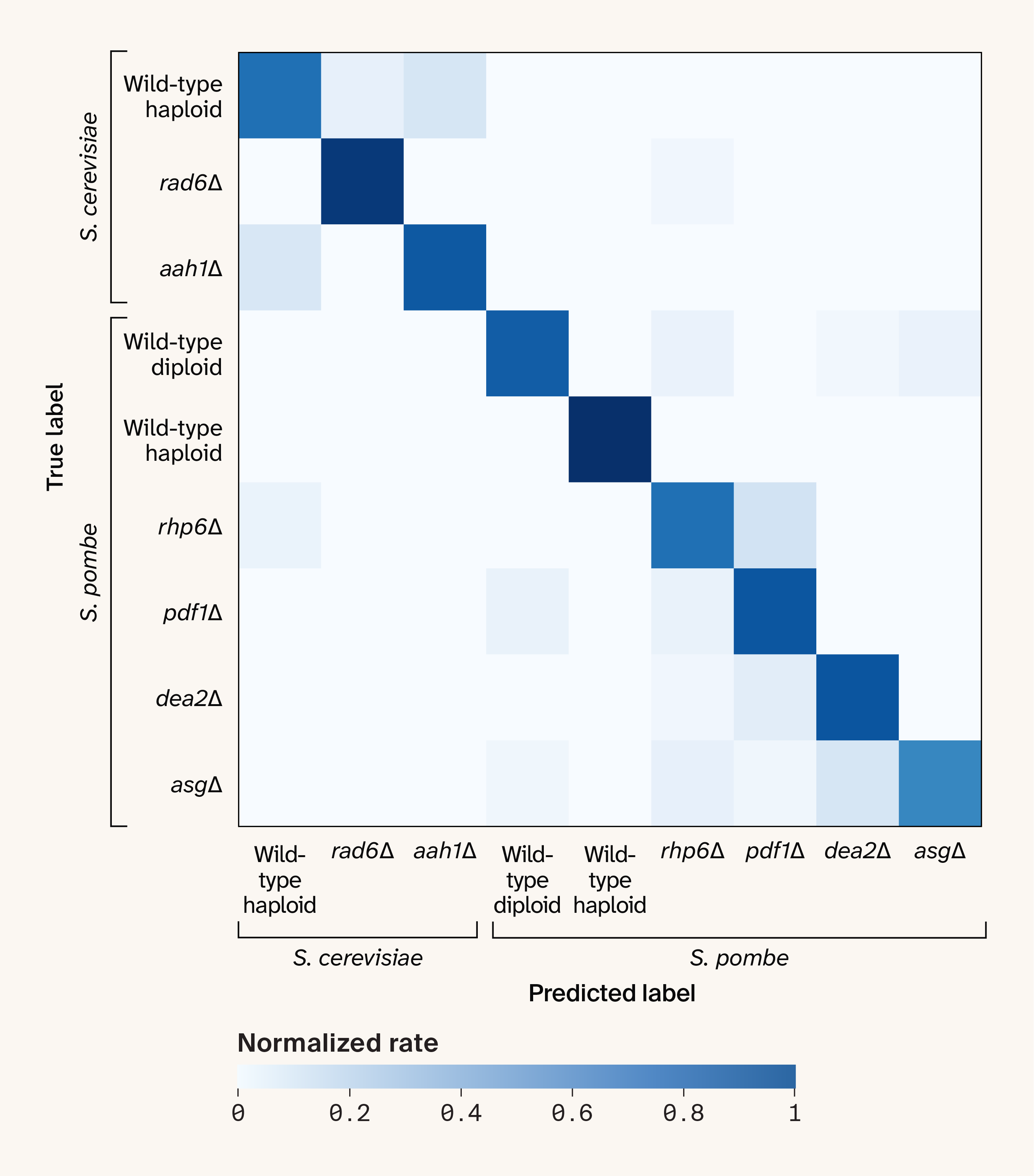
Figure 2. The confusion matrix for strain prediction under standard k-fold cross-validation with five folds.
The cell colors indicate the count of each predicted label for each true label, normalized by the total count of each true label.
Leave-one-plate-out cross-validation reveals batch effects
We then evaluated the same task under leave-one-plate-out cross-validation. The results were substantially worse, with a median MCC of 0.32 (range 0.19–0.42). The confusion matrix revealed that only a few strains remained distinguishable (Figure 3). This result implies that plate-level batch effects dominate whatever strain-level signal exists in the spectra, and that the standard cross-validation approach was effectively overfitting to these batch-specific features. This is possible because each fold in the k-fold cross-validation procedure includes spectra from all three plates, so the model can "see" batch-specific features and use them to help predict strain identity.
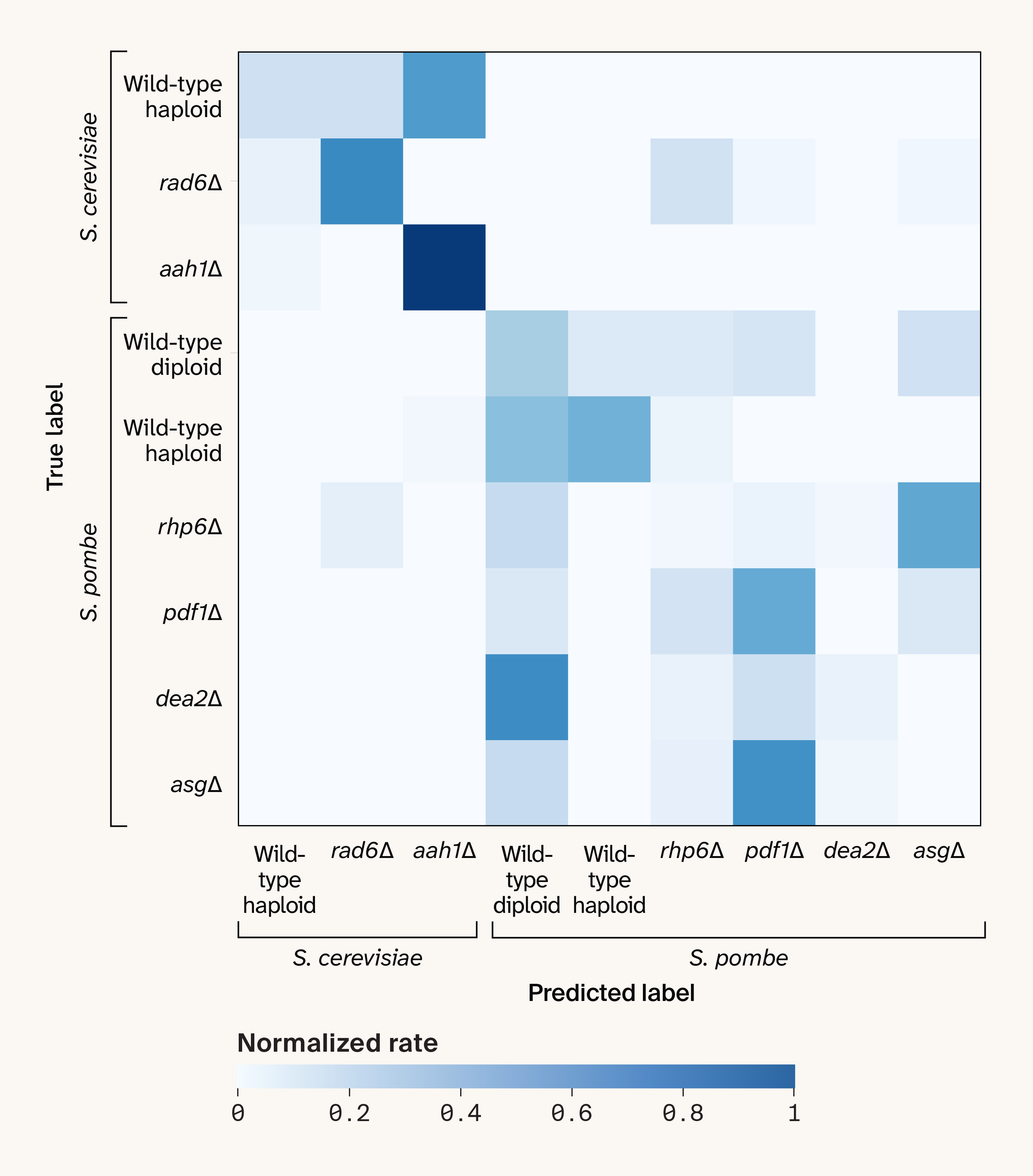
Figure 3. The confusion matrix for strain prediction under leave-one-plate-out cross-validation.
Adversarial prediction of plate identity confirms a plate-level batch effect
We confirmed the existence of a plate-level batch effect by inverting the prediction and cross-validation dimensions: we trained a classifier to predict plate identity instead of strain identity, using leave-one-strain-out cross-validation. We found that the model could very reliably predict the plate from which each spectrum came (Figure 4, A), with a median MCC of 1.0 (range 0.50–1.0). Since the plates correspond to end-to-end replicates of the same experimental protocol, there should be no "true" biological differences between the plates, implying the presence of strong plate-level experimental batch effects that the model is able to exploit.
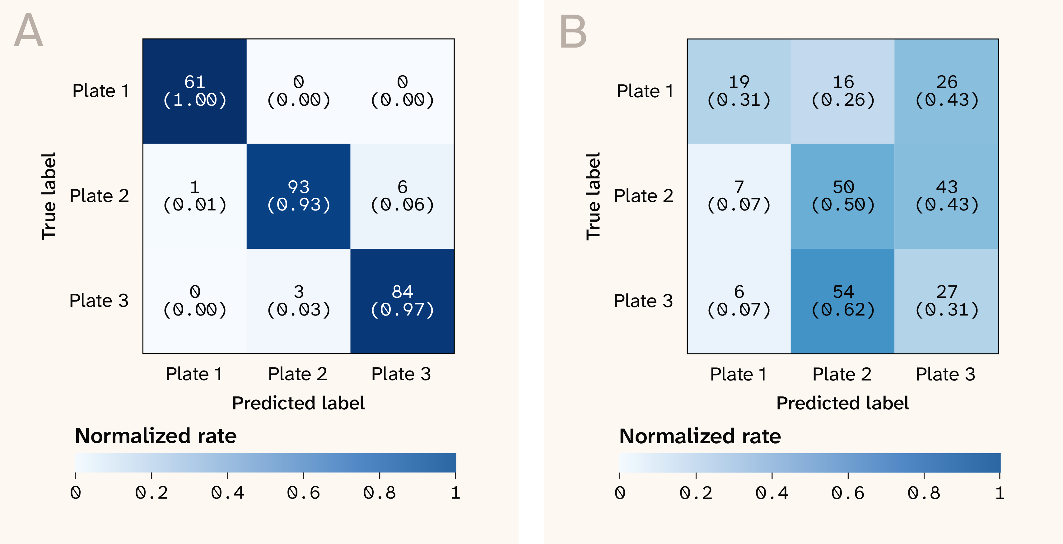
Figure 4. Confusion matrices for predicting plate identity under leave-one-strain-out cross-validation, before (A) and after (B) correcting for batch effects.
Batch correction removed plate-level batch effects but did not improve strain prediction
We applied a linear mixed model to correct for plate-level effects on a per-wavenumber basis (implementation here). After correction, the "adversarial" classifier trained to predict plate identity no longer performed well (Figure 4, B), with a median MCC of 0.10 (range −0.49–0.64), confirming that the plate-level batch effect had been removed. However, strain-level classification wasn’t meaningfully improved (Figure 5), with a median MCC of 0.39 (compared to 0.32 before batch correction). This likely reflects some combination of stochastic sample-level batch effects and genuinely subtle differences between the strains in our dataset that may not result in detectable Raman signatures.
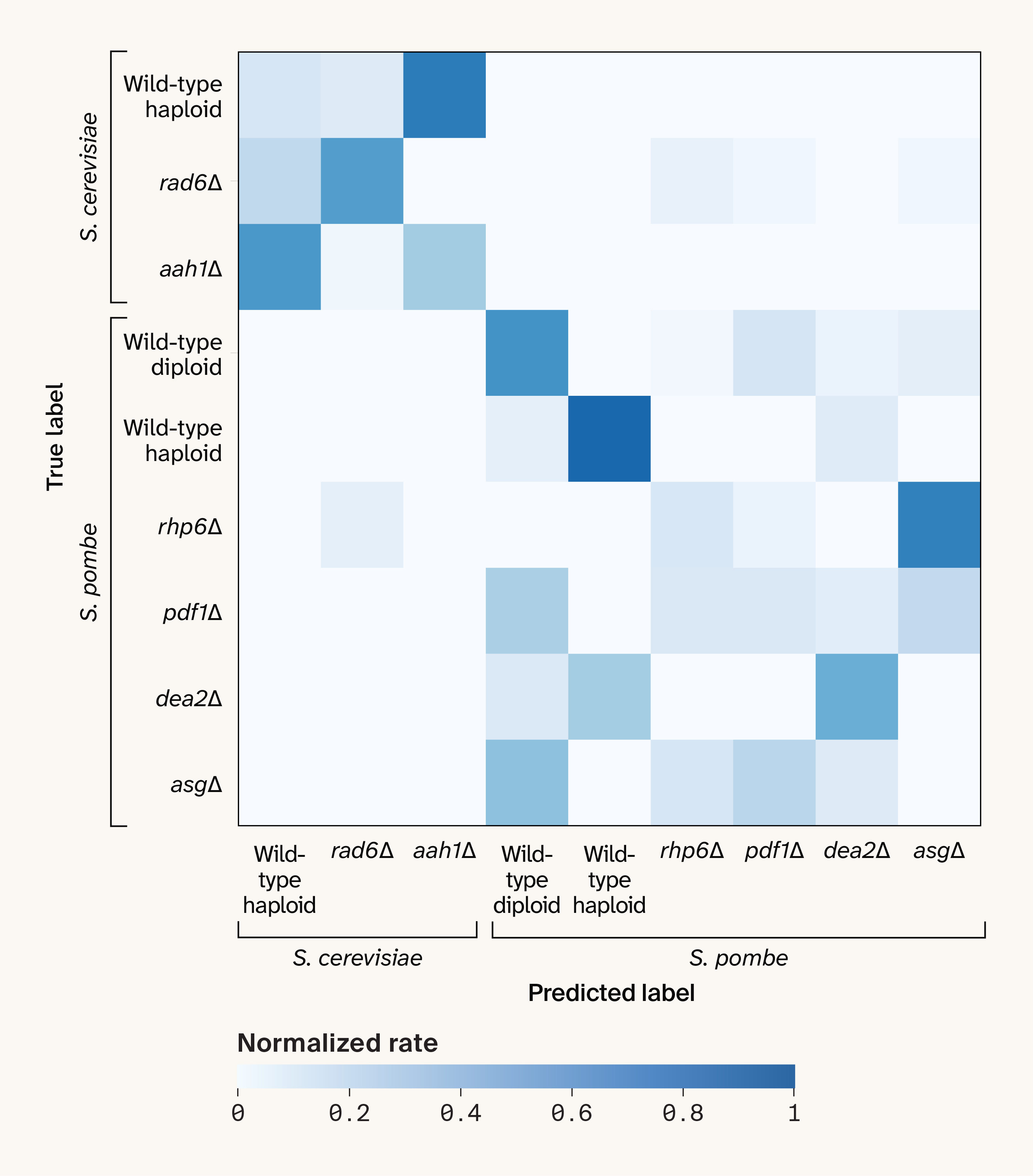
Figure 5. The confusion matrix for strain prediction under leave-one-plate-out cross-validation after correcting for plate-level batch effects.
The cell colors indicate the count of each predicted label for each true label, normalized by the total count of each true label.
Species-level classification works well with or without batch correction
When we shifted from strain-level to species-level classification (S. cerevisiae versus S. pombe), the model performance was nearly perfect under leave-one-plate-out cross-validation (Figure 6). This was true with or without correcting for plate-level batch effects (median MCC of 0.97 without batch correction versus 0.93 with batch correction). This suggests that the spectra contain genuine species-level biological differences that are stronger than the experimental batch effects. Indeed, there was a hint that this was the case in our original strain-level confusion matrix: the misclassifications between strains were predominantly between strains of the same species (Figure 3).
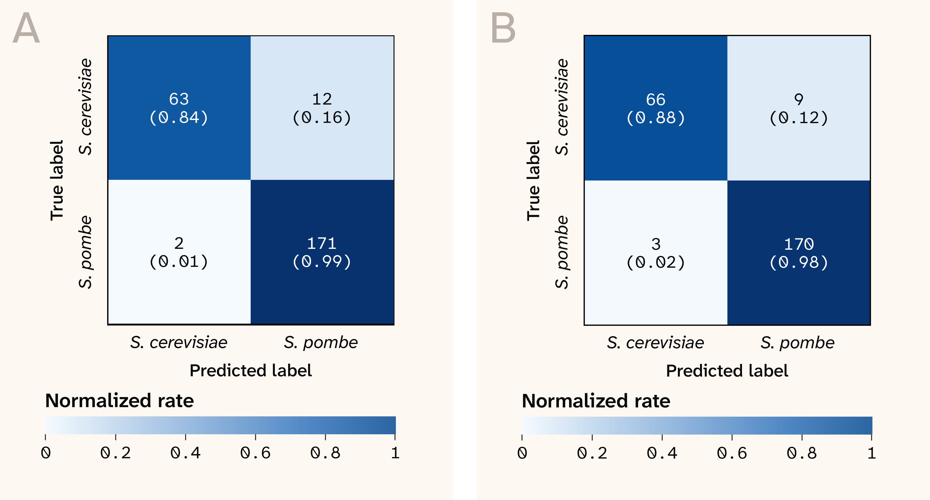
Figure 6. The confusion matrices for predicting species under leave-one-plate-out cross-validation, before (A) and after (B) correcting for batch effects.
As an additional sanity check, we plotted the mean impurity-based feature importances from the trained random forest. We observed that the most important features aligned with wavenumbers at which the mean spectra visibly differed between the two species (Figure 7). This again suggests that the model is leveraging true differences between species that are stronger than the experimental batch effects.
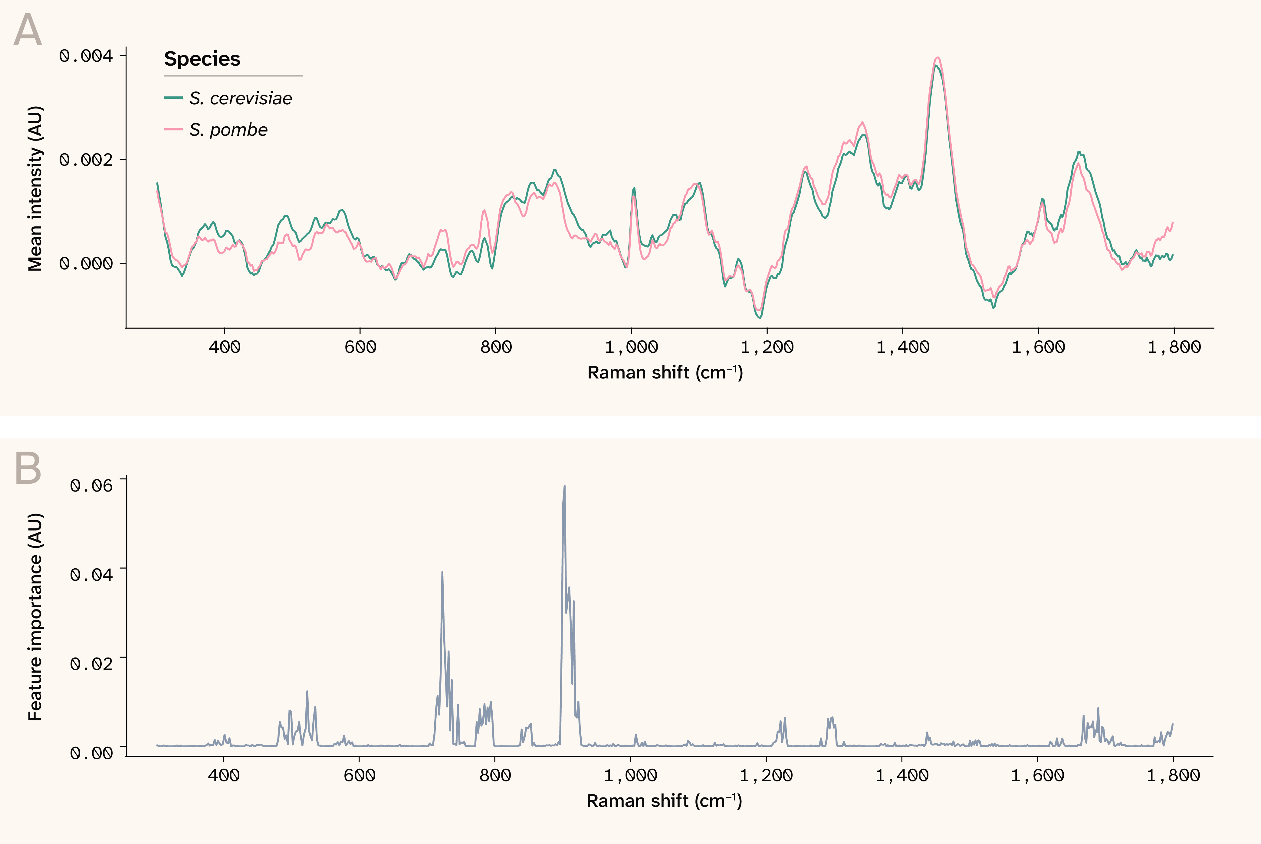
Figure 7. Mean spectra and feature importances for distinguishing between S. cerevisiae and S. pombe.
(A) The mean spectrum for each species, averaged across all plates and strains.
(B) The mean feature importance at each wavenumber from the random forest model trained to predict species identity.
AU: Arbitrary units.
Results aren't sensitive to model type or batch correction method
Finally, to check that our results weren't strongly dependent on our choice of a random forest classifier or our use of a linear mixed model (LMM) for batch correction, we repeated our analysis with both a support vector machine — a conventional nonlinear classifier with a very different architecture from a random forest — and with an established third-party batch-correction method, ComBat. We found that the median MCC values weren't meaningfully different for any combination of batch correction method and classification model (Figure 8).
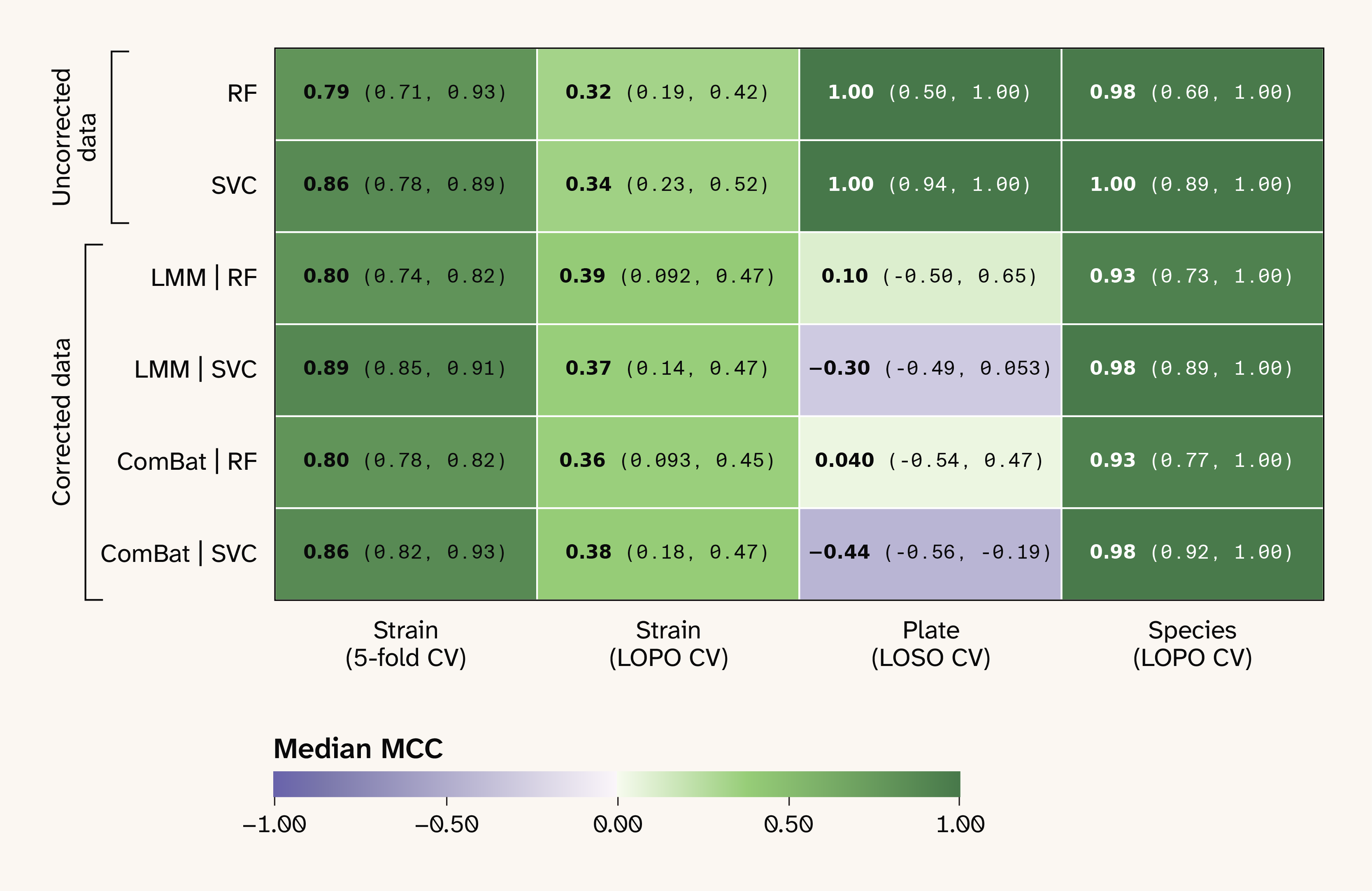
Figure 8. The median MCC values for all combinations of dataset type, model type, prediction task, and cross-validation strategy.
Dataset and model types are shown by row, with prediction tasks by column. The “uncorrected” dataset corresponds to the data without batch correction, and the two “corrected” datasets correspond to data batch-corrected using a linear mixed model (LMM) and ComBat. RF: random forest, SVM: support vector machine, CV: Cross-validation, LOPO: leave-one-plate-out CV, LOSO: leave-one-strain-out CV, MCC: Matthews correlation coefficient.
Limitations and caveats
Several limitations may impact the interpretation of these results. Our dataset itself is small; after QC, we were left with only 248 spectra across nine strains and three plates, yielding noisy cross-validated performance metrics. In addition, the strains in our dataset may be too genetically similar to produce detectable differences in the Raman spectra, so our negative result for strain classification here may not generalize to collections of strains with greater diversity. Finally, the desiccation step in our sample preparation protocol — while necessary to yield a sufficiently strong Raman signal from our spectrometer — is inherently variable and likely contributes to the plate-level batch effect we report here. Other sample preparation techniques may result in weaker batch effects.
We also note that our batch correction approach introduces an implicit train-test leakage, as it applies batch correction once to the full dataset, rather than to each training fold separately. For leave-one-plate-out cross-validation, this effect is severe, as the batch-effect dimension and the cross-validation dimension are identical. This means that our batch-corrected leave-one-plate-out cross-validation estimates are not valid estimates of generalization to fully unseen plates (i.e., plates held out from both batch correction and cross-validation). We instead intend our results to represent a description of how much information about a variable of interest is contained in the spectra, given full knowledge of experimental confounders. In other words, much like PCA or clustering applied to an entire dataset, our batch-corrected cross-validation results describe the batch-corrected structure in the data we have, not the performance we'd expect on new data.
Conclusions
Raman spectroscopy is an extremely sensitive technique. It can detect real, relevant biological signals — and sometimes very subtle ones — but it also readily picks up irrelevant signals associated with experimental conditions. In practice, we have found that Raman spectra invariably contain a mixture of both relevant and irrelevant signals. Because experimental batch effects are a kind of structured noise, standard k-fold cross-validation can give misleadingly good results by allowing models to learn batch-specific features. To distinguish authentic biological signals from batch effects, experiments must therefore include end-to-end replicates, and analysis must be cross-validated on experimentally meaningful batch dimensions. We recommend that experiments incorporate at least three end-to-end replicates from the outset, and that analysis workflows include both leave-one-replicate-out cross-validation and "adversarial" prediction tasks in which a model is trained to predict biologically meaningless variables like replicate or plate identifiers.