Purpose
The following is the outcome of just under a year’s work, carried out under a research contract that called for “a conceptual and exploratory investigation into the potential for protein fibers to perform computational, sensing, or information-encoding functions.” The grandest ambition envisioned at the outset was a set of clear and complete designs for protein-fiber-based devices. After some seven months of poring over the literature, attempting various analytic routes, and occasionally running into dead ends left by gaps in the experimental record or in my own capacities, the final product is rather closer to a partial map of the larger landscape, punctuated throughout by hypotheses, speculations, and design principles. My hope is that the document serves as a jumping-off point for the great deal of work that remains.
The structure of the document is as follows. Chapter 1 lays out a common framework to discuss sensing, transduction, sets out general operating constraints, and closes with a general discussion of protein-based design. Chapter 2 treats transduction, primarily passive, through a minimal fiber model (§2.1.1), a survey of couplings native to protein fibers (§2.2, expanded in Appendix 5), a discussion of figures of merit, bandwidth, and impedance matching (§2.3), and a case study of texture sensing (§2.5). Chapter 3 develops physical reservoir computing as an unconventional modality that may be realizable in protein-based systems, from theory through measurement protocols, material implementation, and open challenges.
Most of the work is yet to be done, and the great majority of it must be experimental. Candidate fibers need to be characterized in the terms the models require. This includes the attainable ranges of the coupling coefficients of Appendix 5, relaxation spectra, the drive amplitude at which response becomes nonlinear, the uniformity of these properties across ostensibly identically constructed devices, and their drift with temperature, hydration, and age. Morphology is left entirely open. The corpuscle model of §2.5 presents one possible design, but whether a layered capsule with the same properties can be fabricated partially or entirely from protein fibers, and how finely those properties can be tuned, remains to be seen. The physical reservoir computing proposal of Chapter 3 also leaves open many questions about morphology and measurement. Many sensors embedded in a synthetic skin is the picture this document hints towards, but a bare mat, a web-like network under pretension, or something very different may serve better. The fading memory and information-processing capacity of a proposed physical reservoir (defined in §3.2.3–3.2.4, with measurement protocols in §3.3.1–3.3.2) offer one basis for choosing among reservoir morphologies and readout designs. The analyses of this document also suggest a number of directions for theoretical work. The visco-piezoelectric model of Appendix 4 is one-dimensional and weakly nonlinear, and as constructed it has a single observable and so cannot act as a physical reservoir (as shown in §3.4.2). The model of Appendix 6 rests on a biological understanding that has since shifted, and there is room to revisit it. Further extending the model to a spatially extended, coupled medium could populate the field formulation of §3.2.2 with the constitutive physics of an actual system, so that the electrode integrals of Eq. (24) could be evaluated on a real strain field, and readout placement could be treated as a design variable in a reservoir-sensing artificial skin platform. Impedance is treated as a lumped-element concept in §2.3.1, and a treatment suited to nonlinear, spatially inhomogeneous, time-varying media would permit further elaboration and analysis of the preliminary sketches of multi-stage devices in §2.4.
Whether a protein fiber-based device can be made to compute in any of the senses developed here remains firmly open. This document offers a vocabulary, a set of models, and clearer idea of what must be measured next. Underlying all of it is a synthesis of several hundred sources across materials science, thermodynamics, mechanobiology, and reservoir computing.
Acknowledgements. This work was financially supported by Speculative Technologies, and was done in collaboration with the Impossible Fibers Lab at Astera Institute, and Impossible Fibers, Inc. I thank Matthew Leighton for constructive feedback on the manuscript, and Wade Ingram for numerous helpful discussions on the lab’s activities. Special thanks are owed to Tim McGee, who provided continuous support and insight over many productive conversations throughout the process.
Jordan Sawchuk
Vancouver, September 2026
1Computation in Physical Systems
1.1Physical computation
“The proper domain of computer science is information processing writ large across all of nature.” – Chris Langton, in Complexity: A Guided Tour by Melanie Mitchell 1
This document explores opportunities and obstacles for protein fiber-based computational devices, in a deliberately broad sense of the word “computational”. This covers a range of ambitions from strictly auxiliary roles (e.g. as a transducer or a sensor) up to intrinsic computation. Most attention is given to the space between these limits, in which the device performs a nontrivial but bounded piece of computational labor. The boundaries between these roles are not sharp, so we must first address a very elementary (but quite challenging) question: When is a physical process a computation?
This question is the subject of a live debate, but the aim here is entirely operational. To avoid the antipodal traps of digital-logic myopia on one hand and pancomputationalism on the other requires an expansive yet structured perspective on computation. What is required is a kind of dictionary between the language of physics and physical processes and the language of computers and algorithms.
1.1.1The abstraction/representation framework
In the Abstraction/Representation (AR) framework,2–4 a physical process becomes a computation when it is used to predict the outcome of an abstract transformation. To motivate the idea, consider the famous example of a slime mold solving a maze, here adapted from Horsman et al.3. If one wants to know the shortest path between two points and in an idealized maze, one could build a physical maze with food sources placed at the physical images of the two points and let the slime mold Physarum grow through it. The organism’s final body shape will trace the solution in the physical maze, from which the abstract answer can be read off. This set-up involved the instantiation of an abstract object (the maze) in a physical system, the evolution of that physical system, and then the measurement and interpretation of the system’s final state as an answer to the question posed. The links between the physical and abstract domains are the essential objects of the AR framework of computation.
This picture is sharper when expressed symbolically. Let be the physical domain and the abstract domain. Then a representation relation and its reverse (instantiation) are maps between a physical system and an abstract domain:
Here is the abstract state represented by the physical state . In the maze example, is the space of idealized mazes, paths, and points, physically instantiated in as real mazes, slime molds, and food sources.
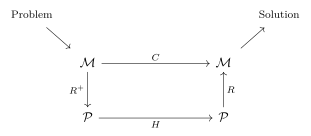
Figure 1. Maps among the abstract and physical domains in the abstraction/representation framework. Based on Fig. 2 from Dale et al. in Ref.5.
Each domain has its own internal evolution. In the abstract domain this is an idealized map carrying the problem to its correct answer, . In the physical domain it is the dynamics . See Fig. 1. The device is a good computer (with respect to the representation relation and the specific problem instance) when the abstract representation of the final physical state is close to the correct answer , i.e., when the diagram 1 commutes within some specified tolerance :
In words,
A computer is (Turing) universal if every computable abstract evolution can be expressed as a composition of primitives for which the diagram of Fig. 1 commutes.2 In a universal machine, commutation is established once, after which the same physical system can be trusted with any computable problem (complexity and resource constraints aside). This is a powerful and rather strict property, but it is not required. A non-universal computer is simply one whose validated diagrams cover a restricted family of problems, and wise operation consists in aligning a physical substrate with the problems it happens to answer well.
Conventional computation populates the same diagram with very different physics than the slime mold.3 For the former, the problem is encoded in binary, perhaps compiled from a high-level language; instantiation initializes the hardware through the full engineering stack (Boolean logic in the transistors, the von Neumann architecture, and so on); the physical evolution proceeds by transistor switching and the charging and discharging of gate capacitances; and decodes the final hardware state into the result . The tolerance absorbs the residual error, e.g. from floating-point round-off. Commutation has been verified compositionally, gate by gate, and computation is universal.
For the slime mold, commutation rests on the empirical observation that Physarum, grown in a two-dimensional domain with obstacles and two food sources, tends to form a minimum-length body connecting them. The minimization is approximate and stochastic, so some error is unavoidable. The slime mold illustrates several ways unconventional computation diverges from the classical picture:
Hardware, software, and input data cannot be cleanly distinguished: the maze is at once the machine and the question. This renders much vocabulary from conventional computing inapplicable.
The computation is consumptive: the organism-maze system answers the question once. Unlike a chip that executes billions of operations before retirement, the cost of construction and programming cannot be amortized over a virtually unbounded number of runs. Other physical computing devices may lie between these extremes. Whether this is a defect or not depends on the application. In implantable biosensors, for instance, one might require a limited lifespan terminated by natural degradation into non-toxic byproducts.
The slime-mold maze solver is non-universal in the extreme, with the validated diagram covering exactly one family of problems.
In summary: a substrate computes only relative to maps between the physical domain and an abstract problem space, and these maps must be specified and validated in advance. A physical computer may be non-universal, and this may be the far more likely case. Finally, a computer is only useful if the user can trust that the diagram commutes for problems whose abstract solutions are not known in advance.
1.1.2Dynamical variables and the I/O map
In any real device, the maps must be realized physically by writing to and reading from particular degrees of freedom of the substrate. For the purposes of model-building, fix a small set of general variables:
- dynamical inputs: the channel through which the environment or an upstream element drives the device during operation;
- internal state variables of the device;
- outputs, whether measured or passed directly to a downstream element;
These specialize the framework of the previous sections to a concrete input/output (I/O) map:
Roughly, the operational content of the instantiation is roughly the preparation of through (and perhaps adjustment of other material parameters); the evolution generates the trajectory , determined by the physics of the device; and the representation is realized by the readout together with its abstract interpretation. For example, might be a force applied to a piezoelectric mat whose polarization state is read off by a voltage developed across the mat. Framing every device in this way puts sensing, transduction, and computation on the same footing. The difference between them lies, at least in part, in the richness of the map .
1.1.3Accessible and information-bearing degrees of freedom
The physical part of the maps and acts primarily through , , and the material parameters governing their coupling to . These collectively form a narrow window onto the full state , so not every feature of the substrate is accessible for computation. Nor is every feature relevant. The information-bearing degrees of freedom (IBDF) are the physical degrees of freedom that carry the computation.
The connection to the representation relation can be made precise. Physical states that agree on their IBDF define equivalence classes, and the quotient of the physical space by IBDF-equivalence is mapped one-to-one onto abstract states.6 never needs to resolve the non-information-bearing degrees of freedom (NIBDF) at all, and a well-chosen representation should be blind to them.
Accessibility and relevance are independent axes. In reservoir computing, the subject of Ch. 3, the great majority of the IBDF are individually inaccessible as the readout is a finite-dimensional, discrete observation of the substrate’s macroscopic behaviour.5 Rather, is required to be an adequate projection of the IBDF retaining enough content to reconstruct the answer (in favorable cases, a sufficient statistic) to within tolerance. The NIBDF manifest as heat and noise and must be managed in aggregate to keep them from interfering with the computation.
1.2Noise & Robustness
Many of the devices contemplated in this document are warm, wet, and small. At physiological temperatures , the thermal energy scale is , comparable to the conformational energy differences that distinguish one functional state of a protein from another.7 Under these operating conditions, thermal noise is a zeroth-order feature of the operating environment which should not be treated as a small perturbation on otherwise deterministic dynamics.8
The phenomena that degrade performance broadly operate on two timescales. Noise refers to rapid stochastic fluctuations entering at every stage of the map (4). The most problematic source of noise depends on the device and its function, and solutions to noise may come with a trade-off. A poled piezoelectric element, for instance, is also pyroelectric, and the influence of ambient temperature fluctuations is indistinguishable from that of mechanical signals. The standard remedy of a subtracting pair of elements to cancel the thermal channel comes at the cost of a second element (§2.3.2). On longer timescales, drift is the systematic change of the device parameters themselves. This may occur through fatigue under cyclic load, or aging at rest, which is characteristic of sensors incorporating organic components.9 Noise blurs individual readouts of a fixed map; drift alters the map itself. In AR terms, both erode the commutation of the diagram 1: noise mainly by increasing the error beyond the tolerance , and drift by invalidating the representation/instantiation maps established at fabrication.
The simplest figure of merit for a noisy readout is the signal-to-noise ratio (SNR). For a scalar readout with mean and fluctuation ,
A viable device maintains adequate SNR across its operating regime, where “adequate” is fixed by the tolerance of the task the device serves.
Robustness is the stability of the map under perturbation. Since the physical evolution is usually stochastic for small devices at ambient temperature, the input history and initial condition do not fix the present state . One might arrange for to report a macroscopic bulk property, so that averaging over the NIBDF yields an effectively deterministic function of the input. In CMOS electronics, for example, energy barriers separate the 0 and 1 macrostates, making thermally activated errors exponentially rare. This protection diminishes as devices shrink, with barriers falling relative to thermal noise once few electrons represent a bit. For this reason, single-electron MOSFETs must be operated at cryogenic temperatures10 unless robustness is recovered at the system level by other means. Consider another illustration from biology: DNA replication withstands the intrinsic noise of the crowded, warm cellular environment through high-fidelity polymerases and kinetic proofreading.7
Disorder itself may be harnessed for robustness. In melanin-like peptide fibers, broadband optical absorption and proton conduction arise from the disordered structure,11 and function that emerges from a disordered ensemble may be relatively tolerant of compositional heterogeneity and manufacturing variability. Function that requires order, on the other hand, may be more fragile. The intrinsic piezoelectricity of protein fibers (§2.2 and App. 5.1.1) scales with molecular alignment, so loss of alignment (i.e., increased disorder) over a device’s service life will degrade performance.
Similarly, noise may be a resource in its own right, e.g. as “a source of free variability” for escaping metastable minima.6 Stochastic resonance is another example, in which noise added to a nonlinear system amplifies sub-threshold signals, so that detection performance is maximized at a nonzero noise intensity.12 The effect is observed in biological sensory systems, where it appears to help organisms register faint stimuli.13
Soft matter systems are typically soft, so protein-fiber devices are liable to mechanical damage. Reported lifespans vary widely: a fish-collagen electrostriction sensor reportedly survived more than cycles over three months with no measurable degradation,14 whereas an electrospun silk/conducting-polymer actuator built by another group lost most of its per-cycle output within a day.15 The ability of biological systems to perform remarkable physical feats with these materials may reflect their metabolic capacity to self-repair. Engineered self-healing has recently been demonstrated in an electroluminescent fiber that recovered roughly of its luminance and remained stable over ten months after being completely severed.16
1.3Thermodynamic and resource constraints
Computation is, of course, bound by the laws of physics. Landauer’s bound is a foundational result which states that, independent of computational modality, irreversibly erasing one bit of information carries an unavoidable free energy cost of (about at ), dissipated as heat.17 Though elegant and universal, Landauer’s bound is not the binding constraint for real devices. Digital CMOS dissipates orders of magnitude above per operation,18–19 and neural signaling is similarly far from the Landauer bound.20
Potentially more relevant are the Bryant–Machta bounds concerning signal transduction.21 Heuristically,
That is, the price of reliable signaling increases with the signal’s tendency to decay in transit and with the noise it must overcome at the readout, and the price decreases with whatever gain the channel can supply. The energetic cost of sending a bit also grows superlinearly with the separation between source and receiver, and the choice of physical channel can matter greatly at very short length scales. Their estimates suggest, for instance, that acoustic signaling is several orders of magnitude more costly than electrical signaling at nanometer scales. Though the qualitative applicability of these results to the present context is somewhat limited by the assumptions on which they rest, it is reasonable to adopt the heuristic that the conversion of a physical state into a readable signal should occur as close as possible to the actual site of sensing or actuation, with minimal structural intermediaries. In brief: transduction and readout should be physically co-located whenever possible.
With regard to a device’s energy requirements, it is useful to distinguish between passive and active materials. A passive material computes using its own equilibrium or near-equilibrium dynamics, drawing no sustained power. A viscoelastic network acting as a convolution filter (e.g. as discussed in Sec. 2.5) performs continuous-time signal processing at zero marginal energy cost per use. The trade-off is that such a device can only offer what its relaxation dynamics afford. It has no gain, cannot sustain a state indefinitely against decay, and it cannot adapt. An active material is held away from equilibrium by a supply of energy (electrical, chemical, or otherwise) and this purchases gain, restoration of decayed states, adaptive reconfiguration, and self-sustained oscillations at a continuous metabolic cost.
Active strategies are central to current proposals of material-based intelligence,22 which naturally raises the question of where the energy is to come from. Protein fibers present an opportunity in this space. Several of the transduction mechanisms surveyed in App. B (dielectric, triboelectric, and some light-coupled mechanisms, for instance) have been studied as means of scavenging power from ambient mechanical or thermal fluctuations. Eliminating the need for an active smart sensor to carry a battery vastly expands the space of possible operating environments.
Finally, energy is just one of a number of commodity resources that must be accounted for in physical computation (e.g. mass, volume, time, precision) and a modality that seems cheap by one accounting may be ruinous by another.23 As a rather extreme demonstration of this, there exists a theoretical design for a DNA computer that could solve hard combinatorial path problems in a small number of steps. However, for any nontrivial problem instance, the mass of DNA required to actually perform the computation would exceed the mass of the earth.24 The massive gain in parallelism simply repackages the problem’s difficulty as a material resource. More relevant (if less spectacular), improving precision tends to be much costlier in analog devices than in digital devices.6 Targeting applications that tolerate low-precision computation might therefore be a sound approach.
1.4Opportunities and challenges in protein design
This document takes the position that a program of protein-based design for computational devices is a worthwhile pursuit. Still, we ought to keep the many challenges in full view, and take care to avoid relying on unsupported (if compelling) arguments in favor of the program.
Consider the available design levers. At the smallest scale, a protein’s material properties are an expression of the sequence of amino acids, often assembled from a modest vocabulary of repeated motifs. Sequences can be written from scratch, existing sequences tweaked in small ways, or motifs can be drawn from unrelated organisms and recombined, presenting an enormous catalogue of properties.25–31 Even without changing the primary structure, supramolecular arrangement, comprising packing, symmetry, cross-link density, and alignment (to name a few) significantly affects the properties of assemblies.32–38 The behavior of an assembly is also strongly influenced by its operating state, such as hydration, ionic environment and loading history.11, 39–41 These levers are strongly entangled. Charged-residue content, for example, governs both the polarization developed under strain27 and the density of proton-transfer pathways.28 This entanglement is an opportunity and a challenge at once. Since each lever controls more than one property, trade-offs abound.35 Performance depends steeply on hydration, which can destabilize crystal phases and shift ionic conductivity by orders of magnitude.11, 41 In many cases, contributions are signed and subtract as readily as they add, with oriented sub-units canceling if improperly aligned. This is implicated at the level of residues26 as well as at the mesoscale, where misalignment of active fibers can result in an inert bulk.36
A single protein or protein-fiber device can host more than one function. Silk-derived -sheet nanostructures have been assembled into a proton-conducting membrane in which the mechanical and conductive roles are carried by the same designed sequence,31 and melanin-like peptide fibers combine broadband optical absorption with proton conduction.11 Synthetic examples include a simultaneously piezoelectric and mechanoluminescent fiber42 and a coaxially spun electroluminescent, magnetically actuatable, and self-healing hydrogel-clad fiber.16 §1.3 argued that transduction and readout should be co-located, and this is satisfied by construction in a device whose sensing and processing elements are one and the same. Such breadth is not, by itself, distinctive. Silicon supports photovoltaic, photoconductive, piezoresistive, thermoelectric, Hall and ion-sensitive responses within a single substrate,9 with a processing maturity no biological material approaches. Rather than a greater number of effects, protein offers the possibility of generating new combinations of properties in one material, among them superior flexibility and biocompatibility.
Still, in the present state of the art, functional properties like piezoelectricity tend to be weak in proteins compared to synthetic devices, and in many reports the noise floor is comparable to the signal being claimed. Measurement of soft matter systems can be difficult, and conflicts in the literature are frequent. Reported coefficients depend strongly on mounting, and outputs are often reported without normalizing to device geometry.43–45 Service life is largely unmeasured, and when reported at all, lifetimes are typically given as a single number based on monochromatic drive at a single amplitude.14–15, 46 This is a thin evidentiary base for a class of material in which aging is expected. Moreover, though often stated as advantages in the literature, economic and environmental claims still precede the evidence.47–48
The case for protein-based design therefore should not rest on beating a ceramic on a coupling coefficient, nor on unexamined appeals to sustainability. Strong arguments in favor of the program remain. For one thing, the design space is large but searchable. A device is specified largely by its sequence, and sequences are enumerable and increasingly screenable before manufacture,25, 49 so design can proceed by search rather than by specification. Further, a small set of levers serves many properties. A process line able to control draw37, applied field38, bath chemistry50 and cross-link density34, 51 can produce a family of distinct devices without being rebuilt for each. This suggests an ambitious manufacturing vision, in which a modest number of control parameters on a common spinning platform yields a broad catalogue of functional fibers, with sequence design and screening carried out upstream at high throughput.
2Transduction
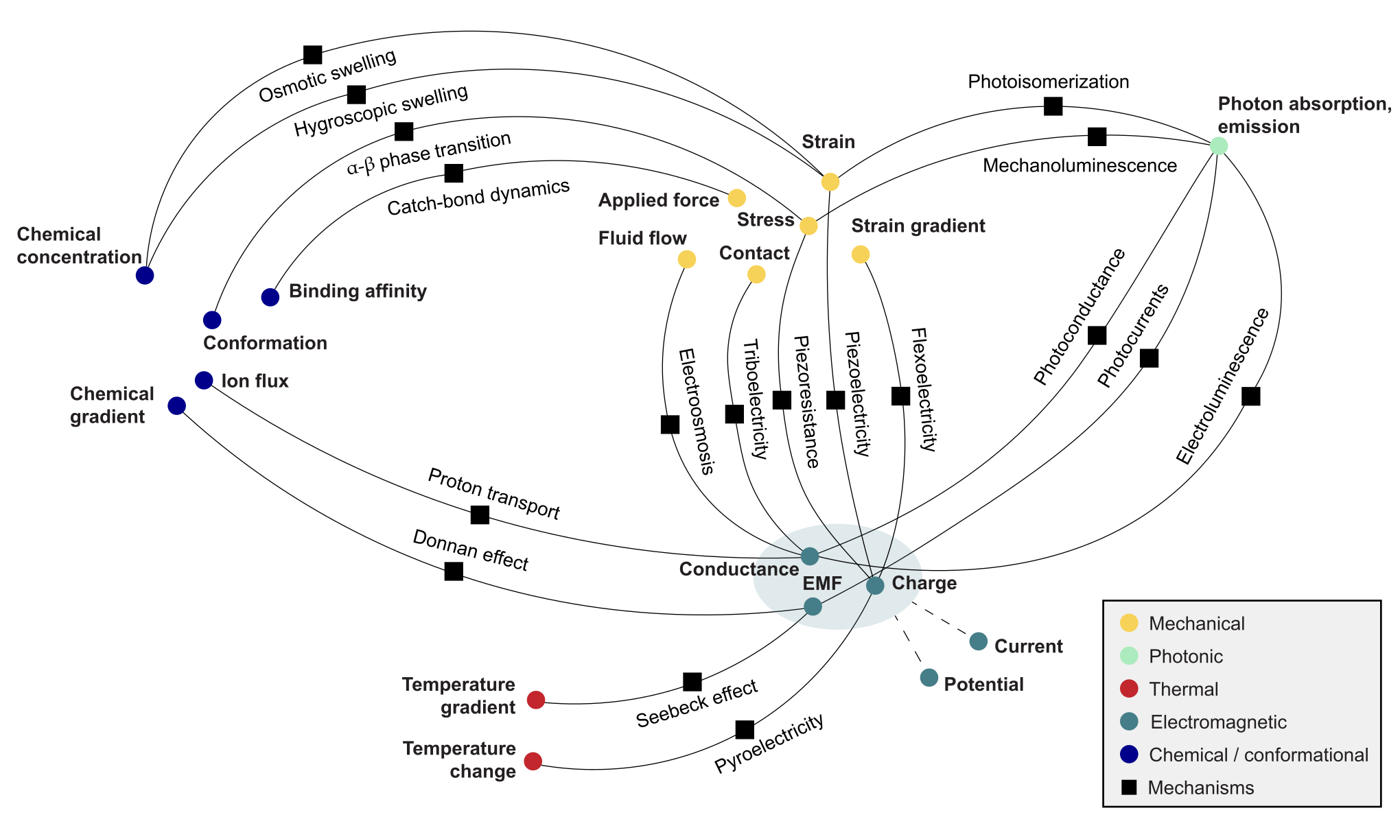
Figure 2. A map of some known transduction mechanisms in protein systems, each of which might be exploited in sensing, signaling, actuation, or computation in a designed device. Not all are equally supported in the literature, nor equally relevant across spatial and temporal scales.
To be useful, a computational system must interface with the world. Signals from the world come in many physical forms, like mechanical stress, temperature, electrical fields, and light. Transduction is, in essence, the conveyance of a signal from one domain to another via a physical coupling that maps a quantity in one domain onto a conjugate quantity in another, say, from applied stress to polarization. Protein fibers exhibit a remarkable breadth of such couplings (Fig. 2).
2.1For / As Computation
The organizing distinction in this chapter is whether a given instance of transduction plays an instrumental or a constitutive role in computation. The instrumental role is transduction for computation. In the language of the I/O map (4), the fiber realizes the input () and/or output () stages, while any nontrivial transformation of information happens in a separate element. A piezoelectric collagen fiber whose voltage output is read only as a faithful copy of the applied strain (we might demand linearity and memorylessness for this application) is operating instrumentally. The constitutive role, on the other hand, is transduction as computation. The transduction event is itself the transformation of interest, so that the information-bearing content of the output is more than a domain-shifted copy of the input. Some degree of distortion is inevitable in physical transduction, so the boundary between these roles is somewhat fuzzy. In the language of §1.1, the distinction rests on the abstract map the device is to be trusted to emulate. If is the identity map (i.e., the goal is perfect transmission) then every departure of the output from a copy of the input contributes to the error. When is nontrivial, the same departure might be information-bearing. A viscoelastic fiber network asked to faithfully transmit strain signals is hysteretic and delayed in its response, poor qualities in a basic transducer! Tuned and read appropriately, those same qualities could perform a passive, frequency-selective computation on the input signal.
2.1.1Minimal model: A nonlinear visco-piezoelectric fiber
To illustrate the constitutive role, I will introduce a one-dimensional weakly nonlinear model of a single fibril exhibiting both viscoelasticity and piezoelectricity. The full construction, from a free energy with internal variables through non-dimensionalization to the open-circuit reduction, is given in Appendix A. The internal unobserved state is described by internal modes representing slow rearrangements of the material (ionic redistributions, etc.) that lag behind the applied strain and field. Each relaxes toward equilibrium as a first-order process with its own time constant, resulting in a discrete relaxation spectrum (often the starting point for viscoelastic modeling52). The model possesses an elastic anharmonicity (stiffness growing with instantaneous strain) and a relaxational anharmonicity (strain-stiffening mediated by internal-mode relaxation on finite timescales). The two are distinguished by their rate dependence, and both have observational precedent: collagen networks stiffen with strain amplitude under quasistatic loading,53 while in ligament tissue the fibril modulus rises with strain rate.54 That the relaxation involves more than one internal timescale is directly supported by Kovacs-like memory effects observed in collagen in the nonlinear regime.55
The fibril is driven by an axial stress and read in open-circuit as a voltage . In dimensionless form, the model reduces to
for strain fixed by mechanical balance [Eq. (48)]. The model is specified by dimensionless numbers, each with a physical reading. Table 2 of App. A defines each and gives its physical reading.
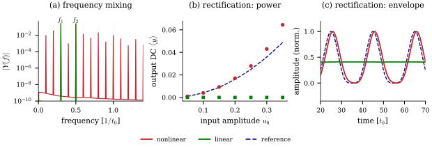
Figure 3. Behaviors of the visco-piezoelectric model with internal modes, comparing the nonlinear model (red) against its linearization (green; identical memory and couplings, nonlinear terms zeroed). Parameters: , , , , , , . (a) Linear and nonlinear spectra for a two-tone input. (b) DC output offset versus single-tone amplitude. (c) Low-passed output for an amplitude-modulated carrier.
Figure 3 demonstrates several behaviors exhibited by the model:
Frequency mixing (heterodyning). Acting on a two-tone input, the quadratic terms produce output components at sum, difference, and harmonic frequencies [Fig. 3(a)]. These are operations underlying modulation, down-conversion, and coincidence detection, though the practical usability depends on conversion efficiency and noise, neither of which is assessed here. For reservoir computing (Ch. 3), the strength and order of mixing correlate with performance across a range of computational tasks.56
Square-law rectification. For a single zero-mean oscillation, the DC component reports the input power [Fig. 3(b)]—a passive, phase-blind intensity meter registering how much vibration is present in a band. For a fast carrier with a slowly changing amplitude, the low-frequency component tracks the squared envelope [Fig. 3(c)]. This is the operation behind the band-power readout of the texture case study [§2.5.4, Eq. (15)].
None of these is available to the linearized fiber, whose response can only relay the frequencies it is given.
The reader should be skeptical: this model has not been validated against real data, and, more damningly, I have neglected thermal noise against my own advice (§1.2). Functional behaviors derived for a noiseless model may completely degrade once noise is introduced. Still, the model demonstrates the general lesson that a property that disqualifies a material as a clean transducer (nonlinearity is in general regarded as an impediment to sensing9) may be the resource that lets it compute. The constitutive view suggests a program of discovery: one examines the intrinsic features of a given material and asks how they might be harnessed. The reservoir-computing paradigm of Ch. 3 is an instance of this program ad extremum.
2.2A survey of transduction mechanisms
Protein-based materials couple the mechanical, thermal, electrical and optical domains in a variety of ways (Fig. 2). Table 1 summarizes these, and App. B treats each in more detail, discussing coefficients, microscopic origins, characterization, and enhancement strategies. Here I highlight some notable features and ideas, and §2.3.2 takes up the corresponding figures of merit at the device level.
Mechanism | Coupling | Representative realization |
|---|---|---|
Piezoelectricity (§5.1.1) | stress polarization | collagen fibrils, peptide nanotubes, electrospun mats |
Pyroelectricity (§5.1.2) | polarization | aortic elastin; poled electrospun PVDF fibers |
Flexoelectricity (§5.1.3) | strain gradient polarization | bone mineral, cell membranes; individual fibrils |
Ferroelectricity (§5.1.4) | switchable polarization | aortic elastin; -glycine crystals |
Triboelectricity (§5.2) | contact charge transfer | electrospun mats, silk-nanoribbon films |
Ionic and protonic conduction (§5.3.1) | field ion current | designed peptide and amyloid fibers |
Electronic conduction (§5.3.2) | field electron current | microbial nanowires, conductively coated fibers |
Piezoresistance (§5.3.3) | strain conductance | composites carrying a conductive phase |
Capacitive transduction (§5.4) | deformation capacitance | ionotronic fibers, hair-like MEMS pillars |
Mechanoluminescence (§5.5.1) | stress light | in electrospun PVDF |
Electroluminescence (§5.5.2) | field light | hydrogel-clad coaxial fibers |
Photomechanical actuation (§5.5.3) | light strain, modulus | azobenzene in spun protein fibers and cellulose fabrics |
Photoconductivity (§5.5.4) | light current | and perovskite composite fibers |
Others (§5.6) | thermoelectric, thermo-mechanical, hygroelectric, chemo-mechanical, chemo-electrical |
Table 1. Transduction mechanisms native to protein-based materials with appendix sections. Hypothetical: motivated by theory but (to my knowledge) not yet demonstrated in a protein fiber.
For each coupling in Table 1, the strength of the material’s response (often characterized by the sensitivity 9) reflects a material’s chemistry and processing, and many design levers recur across mechanisms. Adding a single hydroxyl group to collagen’s building blocks raises the piezoelectric constants by up to two orders of magnitude,26, 30 and carboxylate density governs proton transport in metalloprotein wires.28 Supramolecular order controls the response in amino acid crystals32 and raises ionic conductivity along aligned fibers.29 Piezoelectric polarization is axial, so parallel fibrils add and antiparallel ones cancel; crosslinking-driven self-assembly offers one route to local fibril alignment with a correspondingly enhanced response.34 The impact of water is significant and varied across mechanisms. It lowers the piezoelectric constant of several proteins57 and can drive an irreversible change of crystal phase in glycine,41 while ionic conduction can increase by orders of magnitude from dry to saturated regimes.58 Response is generally tensorial, and geometry determines which components of the coupling tensor are dominant. In chiral polymers the shear piezoelectric coefficients are typically larger than the axial coefficient ,44, 57, 59 so a fiber loaded in pure tension is driven through its weakest coefficient.
As a cautionary note, reported coupling coefficients in the literature differ in tensor component, mechanical boundary condition, drive frequency, and length scale, and few reports are sufficiently explicit about all four.43, 60–61 Coefficients quoted across the literature (and in the appendix) are therefore not directly comparable without great care, and part of the spread attributed to chemistry may be measurement convention.
2.3I/O and Metrics
The pair fixes the I/O character of a device, but whether a given transduction is usable (and whether stages can be chained) is decided by a handful of figures of merit and interface constraints.
2.3.1Bandwidth and impedance matching
Impedance encodes the resistance of a material to external drive, formally described by the frequency-domain pair of conjugate variables whose product is a power, like force and velocity, stress and strain rate, voltage and current, pressure and particle velocity.9 Bandwidth is the window of frequencies over which the device operates as desired, commonly running roughly from the inverse of the slowest internal relaxation time to the inverse of the fastest.
Impedance matching is the problem of getting a signal across a boundary rather than reflecting it. Boundaries are present at the input, output, and any internal stage in a device. For a junction between media of impedance and , power transfer is maximized when the device impedance matches that of the source, since reflection at the junction grows with the ratio in either direction. A device far stiffer than its source barely moves, while one far softer absorbs little of the energy available to it. This is a standard argument for polymer over ceramic transducers in water and tissue.9 In one striking example, a strand of spider silk is so well matched to air that it moves with the surrounding medium at near maximum physical efficiency from 1 Hz to 50 kHz.62 The readout boundary must also be matched. A detector is a load, and a load draws power from the system it is attached to, so a mismatched readout perturbs the state it is meant to observe.
The story is often more complicated, of course. Strain-stiffening,53 crosslink remodeling,51, 63 and temperature and hydration variation41, 57 violate the assumptions of linearity and time-invariance in the standard treatment of impedance. Impedance matching becomes more complicated in this case, with nonlinearities hidden in coefficients which become functions of drive amplitude and operating point.43, 64 Further, impedance is a lumped-element concept, but in many cases (explicitly arising in the modeling demands discussed in Ch. 3) devices must be regarded as spatially distributed systems.
2.3.2Figures of merit
The performance of a device depends not only on its raw coupling coefficients, but also on the geometry, the load, and the readout, and useful figures of merit address these more directly. This subsection collects some principal figures.
2.3.2.1Sensing
For a passive sensor read in open circuit, what matters is the voltage delivered per unit input, so that the magnitude of the raw coefficients can be misleading. In the piezoelectric case (§5.1.1), the relevant figure of merit is the voltage coefficient
A material with modest piezoelectric coefficients but low permittivity can therefore outperform a nominally stronger one in open-circuit voltage per unit stress. The same applies to pyroelectric sensing (§5.1.2). For a device of thickness in its linear regime, a temperature change induces
with the absolute permittivity and the pyroelectric coefficient (both approximated here as scalars along the relevant axis). The amplification of the effect by low permittivity was shown in Ref.65, where a PVDF cell with (far below the strongest ceramics9) produced as its temperature rose from 295 to .
All pyroelectrics are also piezoelectrics,9 and part of the pyroelectric response [the secondary contribution of Eq. (53)] is just the piezoelectric response to thermally induced strain. Molecular dynamics simulations suggest that collagen’s pyroelectric response may be predominantly of this secondary type.59 A pyroelectric element is therefore also a strain sensor, and often an unwelcome one, mechanical disturbance being a primary noise source in pyroelectric detector design. A conventional remedy is to place two identical elements side by side, wired so that their outputs subtract.9 This rejects the mechanical channel, but it is interesting to ponder whether the thermal and mechanical channels might be separable in time instead. In the PVDF cell of Ref. 65, the thermal signal relaxed over finite timescales while the mechanical one was effectively instantaneous. If a fiber’s thermal and mechanical relaxations are sufficiently distinct, a single element might report both, distinguishing a warm touch from a cold one.
Other mechanisms have no internal polarization to read, and must instead modulate an externally supplied signal. For a piezoresistive element (§5.3.3), where strain alters conductance, the relevant figure of merit is the gauge factor
the relative resistance change per unit strain .66 Any such figure holds only within an operating window. Triboelectric output, for example, saturates above a certain pressure, capping the usable range.66
2.3.2.2Actuation and energy harvesting
Where the device is asked to do work, the raw coefficients are misleading in a different way. The units of the piezoelectric coefficient understate achievable actuation, since displacement scales as for device length . Bending actuators amplify the effect further, deflecting a cantilever tip in proportion to curvature length.45 For energy conversion the standard figure is the electromechanical coupling factor , the fraction of elastically stored energy available for conversion to electrical form.43 It appears as the parameter of the minimal model in §2.1.1, evaluated at fixed internal state.
2.3.2.3Comparison across mechanisms
The crudest but most universal figure is the signal-to-noise ratio introduced in §1.2, judged against the tolerance of the task the device serves. Beyond it, comparisons across mechanisms require great care. A useful reference is a review by Homayounfar & Andrew,66 which places the piezoresistive, piezoelectric, capacitive, triboelectric, and transistive families side by side.
2.3.2.4Temporal figures
Where the target application involves processing time-varying signals, relaxation timescales become relevant material parameters. Consider the dielectric couplings of §5.1, for instance. In their linear regime, they are effectively instantaneous and carry no fading memory of their own,61 and in a poled element (one whose domains have been aligned by a strong field during fabrication, like PVDF), maintained stress yields a decaying rather than a sustained output.9 To contribute to temporal computation in a simple passive device, the linear couplings must be paired with a memory-bearing partner. Viscoelastic relaxation supplies the memory of the model in §2.1.1. In an ionic capacitor (§5.4), the double layer and the slow relaxation of the mobile ions that form it lend an otherwise nearly linear geometric element both nonlinearity and memory.67–68 In a triboelectric device (§5.2), the response to a contact event depends on charge left by prior events. This is another presentation of the lessons of §2.1.1: this history dependence both spoils the clean, memoryless sensor and presents a candidate source of the fading memory required by reservoir computing (Ch. 3), provided the charge-relaxation timescale can be characterized and controlled. Additional metrics specific to reservoir computing are developed in Ch. 3.
2.4Composition of mechanisms
In principle, single mechanisms could be composed into richer maps, the output of one stage driving the next. To determine whether an imaginable composition is implementable in reality, one must take a number of things into account. For instance, adjacent stages must be impedance matched, or signal is lost to reflection and heat (§2.3.1). Even where stages are compatible, the thermodynamic cost per bit accumulates stage by stage (§1.3), and by the data-processing inequality, concatenating channels can only degrade the information carried through them.69–70 This sets a real limit on depth, though the per-stage degradation may vary widely across mechanisms and devices, and the utility of such a device depends on whether it can perform its role without the information it discards.
To illustrate the kind of proposal envisioned here, consider a fiber that changes conformation when some ligand binds to it, as in supramolecular fibrillization.63 Suppose that a polarization develops from a strain gradient (§5.1) resulting from the conformational change. This polarization approximately tracks the ligand concentration, , with the dissociation constant setting the gain. The electrode charge is , so the current tracks the temporal derivative . This is recovered only within a band: if varies faster than the electrode charge can leak away, the fiber holds its charge and reports rather than (§2.3.1). If varies faster still than the binding and unbinding kinetics, the fiber reports its own relaxation rather than the stimulus, a failure of the intended function, but not necessarily a useless behavior (§3.2.3). Selectivity is a separate problem in such a sensor.71
This idea warrants closer scrutiny than I have been able to give it. Generic models of this kind, with an explicit accounting of noise and of the material parameters that set the operating bands, may be a low-barrier avenue for experimentally testable theory, perhaps following the information rate analysis of Mattingly et al.70
2.5Case study: Sensing textures
This chapter closes with a case study of a bio-inspired texture-sensing platform. The goal is to extract information about a surface’s fine textural detail by dragging a small, soft contact across it. This is how humans perceive such details: when we sweep a fingertip across a surface, features below m are resolved not as a spatial pattern of pressure but as the vibration generated by the sliding contact.72–73 The analysis builds on a classical model of a biological mechanoreceptor as a mechanical pre-processor. Challenges unmet by the simple transduction picture will motivate the reservoir-sensing perspective of Ch. 3.
2.5.1Texture and the scanning drive
A device senses some property of the environment if, through the stimulus , that property can be inferred (or decoded) from the readout . The first task is to determine which abstract qualities of a surface encompass its “texture”. Here, I identify texture with the roughness of a surface, defined as follows.
Let be a zero-mean height field along a one-dimensional scan track of a surface. Assuming statistical stationarity of the profile, the second-order structure of the surface is captured by the power spectral density74
For example, a regular corrugation of amplitude and peak-to-peak distance has height field , autocovariance and hence PSD , a single spectral line at the corrugation wavenumber . Real surfaces have a continuous spectrum.
The sensor moves a small contact along the scan track at velocity , converting the spatial profile into a time series in which each wavenumber appears at angular frequency
so the same feature of wavelength can arrive at the transducer at a frequency set jointly by the surface and the sensor’s motion.
Take scanning speeds of order cm/s and fine features of wavelength . Then the information-bearing content of the drive arrives at frequencies Hz, with typical presentations concentrated in roughly 50– Hz. The force carried by these fine textural details will be much weaker than the static or slow forces from the contact.75
2.5.2LS model: A mechanical high-pass filter
The Pacinian corpuscle is a sub-dermal biological mechanoreceptor approximately 2 mm in length, consisting of 50 concentric layers (lamellae) wrapped around an afferent terminal. It is responsible for discriminating fine texture, responsive in the 40–1000 Hz band, with a peak sensitivity in 250–550 Hz76–77 [Fig. 4(a)]. In the Loewenstein–Skalak (LS) model [Fig. 4(b)], the capsule acts as a passive mechanical high-pass filter, pre-processing vibrations from exploratory touch so that only vibrations carrying fine textural information reach the afferent, the sensory nerve fiber whose terminal sits at the core of the capsule and carries the resulting spike train to the central nervous system.
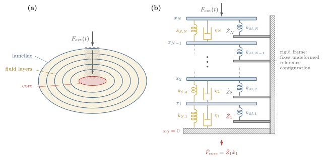
Figure 4. (a) Concentric lamellae and fluid layers surround the core, which contains a demyelinated neuron. The gray box marks the slice examined in the LS model. (b) Spring–dashpot representation of the LS model. These figures are based roughly on Figs. 1 and 4 of Ref.78.
The model treats the th lamella as an elastic membrane of stiffness , coupled to its neighbours by Kelvin–Voigt elements with stiffness and damping [Fig. 4(b)]. The resulting system in frequency space is solved in App. 6.1 for the transfer function
where is the tridiagonal matrix of inter-layer couplings [Eq. (58)]. The right-most expression is read intuitively as the impedance of the final fluid layer times the complex admittance carrying mechanical signals from layer to layer 1.
The capsule behaves as a high-pass filter (the mechanism and its scaling with lamella number and stiffness ratio is analyzed in App. 6.1). At low frequencies, the viscous fluid stays in equilibrium with the applied force, so each fluid layer acts as a spring, passing only the fraction of its outer neighbour’s displacement inward. Static transmission is therefore suppressed geometrically with the number of lamellae as (62). At high frequencies, the dashpots rigidify so the stack translates as a rigid body, transmitting the signal perfectly [ as ]. Between these two limits, the capsule differentiates the signal [], reporting the rate of loading (60).
For texture sensing, this kind of mechanical pre-filtering would help keep irrelevant information from swamping the readout. Given the right elasticity and viscosity of the membranes and fluid layers, signals from static contact forces are suppressed while vibrations from fine texture arrive in the differentiating band and are passed to the transducer at the core. The bands are set by the ratio and the number of layers , both morphological parameters tunable in designed materials.
2.5.3Embedding in a synthetic skin
Consider now a corpuscle-like element embedded below the surface of a synthetic skin. It may be one of many such receptors harvesting information from the same contact patch. Describe this contact by a weighting kernel translating at speed . For simplicity, I assume this to be fixed, symmetric, and of unit gain, so the resulting kinematic drive and its temporal power-density spectrum are
The finite patch acts as a spatial low-pass that erases wavelengths much shorter than its width, and the scan converts wavenumber to frequency via Eq. (12).
Between this drive and the capsule sit two further mechanical elements: the local skin patch and the bulk tissue, treated here respectively as a mass–spring–damper and a simple Kelvin–Voigt element coupling the patch to the outermost lamella. Since each element is linear and time-invariant, the skin patch model can be simply appended to the ladder of Fig. 4(b) as an th rung. Solving the extended ladder (App. 6.2) factorizes the total response exactly into skin, coupling, and capsule stages [Eq. (70)], delivering the spectrum to the transducer at the core. The full chain can be matched to the texture band to ensure that the right signal is passed to the core [Fig. 7]. A receptor that is compliant relative to the patch reads the skin’s motion without perturbing it [App. 6.2], so that many receptors with distinct transfer functions could be embedded in the skin.
2.5.4Readout
The readout is the stage that converts the mechanical state at the core into whatever kind of signal the downstream elements require. This could be a vector of observables read at several sites, or a signal evolving in time. The afferent’s output in a Pacinian corpuscle is the latter, sending a spike train to the central nervous system, the textural information encoded in its temporal structure.79–80 Let us consider the much simpler case of a scalar readout, i.e., a single transducer at the core reporting one number. A natural passive choice, consistent with some empirical observations of the Pacinian corpuscle,73 is the power registered in the responsive band, read through the transducer’s sensitivity band :
What information does carry about the surface? Substituting Eq. (14) and making a change of variables ,
The readout is therefore a weighted moment of the surface spectrum, through a window rescaled by the scanning speed . If over the supported band, for instance, then the th spectral moment of the surface. Then a manifestly speed-invariant scaling is , for which is the displacement variance. For natural surfaces (, §2.5.1) this is dominated by coarse features, so such a readout might be nearly blind to fine texture. For , is the velocity variance. This suppresses the coarse features but is strongly speed-dependent, and in general, increasing increases the sensitivity to fine structure while simultaneously increasing the speed-dependence of the output. Where the total weight is not approximated by a power law, as in some regimes of the bandpass developed in this section and App. C, changing the scanning speed reshapes the sampled band rather than just rescaling . See Fig. 5.
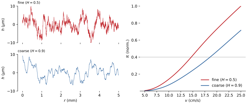
Figure 5. Left: 5 mm sections of two synthetic surfaces with RMS height 4 m and spectra , flat below and self-affine above it.74, 81 The Hurst exponent sets how much of that height sits in fine features, so is the rougher surface and the smoother. Right: Normalized band-power readout (15) as a function of scanning speed , computed via (16) with the embedded transfer function plotted in Fig. 7 with a Gaussian contact kernel of width m and a flat, memoryless transducer window over 10–2000 Hz. The readout correctly ranks the fine surface as rougher at every speed, but both curves climb steeply with , and their ratio drifts as the window slides across the two spectra. The ambiguity is marked as the horizontal gray line: the output for a fine surface scanned at cm/s matches that of the coarse surface scanned at cm/s.
A partial passive fix is to build a known length into the sensor. A fixed surface periodicity (as in human fingerprints) stamps a reference line into the spectrum whose measured frequency may be used to infer directly.82 This requires a single clean reference and a stationary spectrum, but every assumption built into the model (linear contact, stationary statistics, etc.) degrades under natural, active exploration.74, 83 Embedding many receptors in a synthetic skin (§2.5.3) adds channels but does not obviously resolve the issue. Without an independent measure of , recovering from seems to require a nonlinear map from the drive’s history to a label. This (together with the biological precedent noted above) suggests that the computation should be treated as a fundamentally temporal one. The next chapter develops physical reservoir computing, a framework for processing time-varying signals in the intrinsic dynamics of materials.
3Reservoir computing
3.1Introduction and abbreviated history
Reservoir computing (RC) is a computational paradigm based on recurrent neural networks (RNNs) in which a fixed dynamical system (the reservoir) is driven by an input signal , its state is observed, and a trained readout maps the observation to an output . The nonlinear embedding of the input signal into the high-dimensional state space of the reservoir renders otherwise inseparable inputs linearly separable, so that only a memoryless readout (often a simple linear perceptron) needs to be trained. The theory of RC has mostly developed around digital implementations, but in principle any sufficiently rich input-driven dynamical system can act as the reservoir. Computation that exploits the intrinsic dynamics of a physical system is called physical reservoir computing (PRC). Realizations of PRC have been reported in photonic, electronic, spintronic, mechanical, fluidic, chemical, and biological substrates.84–86
The approximation on which the paradigm rests precedes it by some fifteen years, stated in the language of nonlinear systems theory. The fundamental objects are causal time-invariant operators, or filters in the engineering jargon. Boyd was interested in approximating arbitrary filters by Volterra series.87 For our purposes, these filters are computations we want to design a physical system to perform. Some examples of filters include: the pure delay , which asks the system to report on the inputs time steps in the past; products , which ask it to combine information from two separate moments of the past; and, more generally, reporting the solution of a nonlinear ODE driven by . These tasks reappear in §3.2.4 as test functions against which the information-processing capacity of a physical reservoir can be measured.
Boyd proved that any time-invariant filter with fading memory can be uniformly approximated by a bank of parallel linear filters that separates points in the space of input histories, followed by a static memoryless nonlinearity. Concretely, in the single-input single-output case, a nonlinear readout of a linear dynamical system can always be made to approximate a desired filter . The coordinates of that system are themselves the filter bank,
each kernel decaying exponentially for stable . The bank acts as a basis: each coordinate reduces the input history to a single number at time , so they collectively implement a feature map from driving histories to points in , with the separation condition ensuring that distinct histories can be told apart. Since the bank does not depend on the target, what remains is to train the static nonlinearity (a regression on ). More recent work has shown that, subject to a few technical conditions, a wide class of dynamical systems (including nonlinear ones) can take the place of the linear filter bank. Moreover, a suitable dynamical system can serve many filters at once, with each target needing only its own readout function .
This structure was rederived in the early 2000s, twice and independently. Jaeger, observed that it was possible to skip the unstable and costly process of training RNNs, and simply train the output weights of a random RNN. The network need only satisfy what Jaeger called the “echo state property”, in essence Boyd’s fading memory. Reservoirs based on this framework are called echo-state networks (ESNs).88 Around the same time, Maass, Natschlager, and Markram, modeling cortical microcircuits, introduced the liquid state machine (LSM): a more generic recurrent medium driven by a continuous input stream and read by a memoryless function.89
Within a year of the LSM’s introduction, Fernando and Sojakka provided a vivid and rather literal physical demonstration of the concept.90 In their paper “Pattern recognition in a bucket”, they report the following set-up. Motors at the rim of a tank of water transduced inputs (binary values for an XOR task, frequency components of the spoken words “zero” and “one” for a speech task) into agitations of the surface. A camera recorded the resulting interference pattern (the reservoir state) and 50 perceptrons in parallel were trained on the coarsened vectors of pixel values. The raw inputs are linearly inseparable, so a perceptron alone could not perform the task. By first embedding the signals in a high-dimensional space via the nonlinear, temporal mixing of the water, a linear classifier was able to discriminate the inputs. Physical realizations have since been reported in a range of substrates, including organic electrochemical networks,91 self-organizing nanowire / memristive networks,92 passive photonic cavities,93 the body dynamics of a soft robotic arm,94 liquid egg albumen,95 and beads of wine.96
Theory has continued to develop alongside physical demonstrations. Universality has been established for the discrete-time ESN97 and for generic networks of nonlinear springs and dampers,98 and extended to unbounded stochastic inputs and target filters without fading memory (with approximation defined in an sense rather than uniform).99 The information-processing capacity of a fading-memory system was shown to be set by the number of linearly independent observed state variables, establishing a trade-off between memory and expressiveness.100 Using delay lines, both the network101 and the physical reservoir itself102 have proven dispensable in some architectures.
3.2Theory: Models and core metrics
To keep this document reasonably self-contained, this section lays out the essential theoretical concepts. I begin with echo-state networks, the most developed of the theoretical models, and then generalize the picture to accommodate physical substrates. The presentation herein is far from comprehensive, but reservoir computing is an active and growing field, and there are a number of excellent texts and reviews worth consulting.
3.2.1Echo-state networks
Let be a -dimensional input signal, the state of the internal network units, and the output. Time is discrete: . Following Jaeger, the state is updated as
where is a component-wise nonlinearity and and are fixed random matrices. The output weights are to be trained.88 For simplicity, feedback and feedthrough are neglected ( is independent of , and depends on only through ), and the readout is memoryless.
The system is said to have echo states if is uniquely determined by the left-infinite input sequence . That is, the state is an echo of past inputs, with any influence of the initial condition washed out. Without this property the same input can yield different readouts depending on an unobservable history, rendering the dynamics irreproducible. When the property holds, the activation of each unit is (after an initial transient) a function of the input history alone,
the function called the echo function of the th unit. These are the parallel fading-memory filters of Boyd’s theorem realized in artificial neurons. A sufficiently inhomogeneous network furnishes a rich bank of distinct echo functions, or in Jaeger’s words, “a rich reservoir of dynamics ‘tapped’ by the output weights.”88
Given a target filter , one drives the network with a training input, records the resulting states, and fits the output weights so that approximates over a training record . In practice this is a least-squares fit with a regularization parameter , or ridge regression:
Collecting the states and targets column-wise into and , the closed-form expression for the minimizer is a single solve:
3.2.2A formulation for physical reservoirs
Physically implementing a reservoir computer in a soft matter system requires a more general picture. The formulation that follows is my own, though it is assembled from standard ingredients and takes inspiration from prior work. Describe the reservoir state by a field on a spatial domain in some state space with nonlinear, dissipative, autonomous, Markovian dynamics described by an abstract operator . In many cases of interest, the inputs will have spatial extent, too. Describe the drive by a field on an input region , say a contact patch or a boundary. Then
where is an operator carrying the input field to a forcing field. The state is observed through a finite set of numbers fixed by a measurement map
with measurement noise . In many cases, will be a linear functional
with instrument profile fixed by the construction of the device. For example, the charge collected by an electrode deposited on a piezoelectric layer integrates the stress over the electrode footprint,9
so is the footprint itself. The profile needn’t coincide with the sensor’s footprint: in a four-electrode resistive measurement, it is set by the current paths through the material. Then the impedance measured between a current-carrying pair and a potential pick-up pair is103
the resistivity field integrated against a sensitivity field extending well beyond the electrodes themselves.
As before, a readout is trained to approximate the desired filter by fitting the weights in , possibly by the ridge regression (20). The full chain is then
where the maps , , and are fixed by the physics of the hardware, and the final stage is trained. The ESN of §3.2.1 is recovered as the special case in which the “field” is the vector of unit activations on a discrete set of nodes, time is discretized, , applies both the recurrent mixing and nonlinearity, and the state is observed completely and noiselessly ().
When the fading-memory requirement is satisfied, each observable becomes a functional of the drive history once initial transients have decayed, generalizing the echo functions of §3.2.1. Each is a composite of the input coupling , the reservoir dynamics , and the measurement , and it is this composition that constitutes the filter bank. The upshot is that the number and placement of contacts, the instrument profiles they present, and the nature of the input coupling are all aspects of reservoir design. Readout number and placement have received some attention recently,104–106 but general design principles are lacking. Fortunately, adjusting the readout (say, repatterning an electrode layer) is a relatively cheap way to explore a material’s computational capacity.104
The next sections address fading memory and the capacity measures that quantify expressivity. In the physical framing developed here, both are properties of the composite rather than of any single stage. No stage may violate fading memory, whereas the nonlinearity on which capacity depends need only be supplied by one of them. Where it is supplied is a design choice, and §3.4.1 surveys the physical options available at each stage.
3.2.3Fading memory
An operator has fading memory (FM) if inputs that agree over the recent past produce similar outputs in the present. Boyd makes this precise as follows.87 Let be decreasing with , and define the weighted norm on input histories
A filter has fading memory with weighting function if it is continuous with respect to the norm (28). That is, for every there is a such that implies . Since , this is strictly stronger than ordinary continuity. An exponential describes a system ‘forgetting’ on a timescale , so is the formal counterpart of the relaxation spectrum of §2.3.1. Boyd’s example of a filter that does not possess fading memory is the peak-hold operator , which is continuous but retains a single past event indefinitely, so that no choice of weights can render the remote past negligible.
Physically, fading memory is a statement about dissipation. A system forgets its initial condition only by contracting volumes in state space, which Liouville’s theorem forbids in purely Hamiltonian evolution. Fading memory can also fail when a driven material keeps a permanent record via plastic deformation, ferroelectric switching, or any hysteretic branch structure that leaves the response dependent on an unobservable history.
Fading memory says that a system forgets, but nothing about how fast. For universality proofs, the relaxation time is irrelevant,97 but in a real device it is a crucial consideration. Consider the single-input, single-output pure delay task , . The input at lag survives in the state with magnitude for contraction rate , while the readout noise sits at a floor . The recoverable delay is therefore bounded by the noise floor,
The accessible timescales are set by the relaxation spectrum, a manufacturing variable, and as explained below, faster forgetting (smaller ) buys sharper separation of recent signals at the cost of memory depth.
3.2.4Information processing capacity
A reservoir well-suited to one task may be poorly suited to another. The capacity of a reservoir is a task-specific metric that quantifies how much of a given target a linear readout of the observables can actually recover. Let be any target functional of the input history, e.g. a delayed copy of the input, a product of inputs at past times, or the solution of a non-autonomous nonlinear ODE with inputs . Drive the system with an i.i.d. input and fit by least squares. The capacity for that target is the fraction of its variance that the readout recovers:
A value means perfect reconstruction, and means that the observables contain nothing of .100 Evaluating on a complete, orthogonal family of functionals (commonly products of Legendre polynomials of the input at various lags) and summing gives the total information processing capacity . Dambre and co-workers proved that for a system with observables ,
with equality when the system has fading memory and the observables are linearly independent. A reservoir with observables therefore has a fixed amount of capacity to allocate among different tasks, enumerated in the basis functionals. Conventionally, the capacity is split into memory capacity and nonlinearity. Memory capacity is measured against the delay tasks:
The curve versus lag is the forgetting curve, and (29) is made precise and measurable by identifying the lag at which the forgetting curve reaches the noise floor. Nonlinearity is measured against higher-degree targets (typically products of inputs at distinct past times) and captures the ability to compute polynomial mixtures of the input history. For linearly independent observables, (31) gives a memory–nonlinearity trade-off
where is the nonlinear capacity. In words, this says that any capacity allocated to nonlinear functionals is unavailable for linear recall, so a system driven harder into its nonlinear regime loses memory depth as it gains expressiveness.100, 107 The trade-off is easiest to see in a single observable. Suppose for i.i.d. zero-mean input . The product term is noise to a linear readout attempting to recall , and decreases as grows. The capacity lost is reallocated, reappearing as , and the total stays at one.
A division of labor is one response to this trade-off: in a heterogeneous reservoir, a near-linear subsystem may retain memory, while a nonlinear subsystem transforms it.107–108 The same division can be accomplished in a spatially extended substrate, with spatially varying memory and nonlinearity within one material. The placement and profile of the measuring instruments then select the mixture seen by the readout.104
3.3Measurement protocols and benchmarks
3.3.1Estimating capacities
The capacity (30) can be estimated from empirical correlations. Let be observables measured at times for the system under some driving, with taken after washout of any transients from initialization. The observation correlation matrix is defined as
Then the least-squares capacity for some target (zero-mean, WLOG) can be estimated by
where is the target-observable correlation. For example, for the -step delay-recall task, . Equation (35) can be read as the fraction of the target’s variance recovered by projecting it onto the recorded observables. Since depends only on the device and the drive, it can be collected just once and computed across many different targets.
The estimator (35) is biased to inflate capacity on finite records due to chance correlations. Over a large basis, these spurious correlations can significantly overestimate capacity.100 One way to address this is to build an empirical null (e.g. a target built from an independently drawn input record) and zero any capacity that does not exceed the null before summing.
The bound in Eq. (31) counts linearly independent observables only. When the correlation matrix does not have full rank, the inverse in Eq. (35) is replaced by the pseudoinverse, and the total capacity is bounded by rather than by the nominal channel count.100 Observables drawn from a spatially extended substrate will always be correlated to some degree, with dense readout arrays found to be strongly co-linear in practice.105 The eigenvalue spectrum of is therefore a task-agnostic measure of how many independent observables a device actually has over a given input range. A tail of eigenvalues at or below the noise floor indicates that some transducers may need to be repositioned. Redundancy is not necessarily wasted, however, as averaging correlated channels suppresses the measurement noise on the dominant modes.
3.3.2Measuring fading memory
Pulse–relaxation data is one way to probe the memory of a material: apply a delta-like input and record the return of the observables to baseline, reading the relaxation timescales from the measured curve. This is useful for identifying accessible timescales and is suggestive of fading memory, but it does not on its own demonstrate convergence under a sustained drive.
Another approach is to drive the device with two distinct conditioning sequences , on and then apply the same drive to both for , recording the observables and . If the two response records converge to within some noise floor and stay there, the device has fading memory over that drive. If they settle onto persistently different responses, it does not.109 The rate at which converges to the noise floor as estimates the conditional Lyapunov exponent of the driven system.107 Note that a material that has fading memory at small drive can exhibit hysteresis for large drives, so the result is a property of the operating regime, and tests should be run at the amplitudes and frequencies relevant to the target application.
Lastly, the capacity measurements of §3.3.1 can provide evidence of fading memory. The forgetting curve ( as a function of the lag ) is near unity for small and then decays to the empirical null as increases for a device with fading memory. Moreover, by the equality condition of Eq. (31), a total capacity approaching is attainable only by a system with fading memory, so a saturated or near-saturated capacity provides evidence (albeit limited evidence) of fading memory.100
3.3.3Benchmarks
A conventional battery of tasks for quantifying the performance of reservoir computers exists, which have the virtue of comparability with the literature. A tutorial review and critique of standard benchmarks is given by Wringe and coworkers.110 The most common of these are described below.
Delay recall and polynomial probes are the capacity measurements already described. Parity tasks (typically ) demand both memory and nonlinearity jointly. The NARMA- family111 tests emulation of a mildly nonlinear system with -step memory:
This is the de facto standard test in the RC literature, though parameter values vary widely across reports and the recursion can diverge.110 Chaotic time-series prediction (Mackey–Glass, Santa Fe laser) and spoken-digit classification are also standard. At least two open-source standardizations of this battery have been developed. RCbench112 computes memory capacity, NARMA-, kernel and generalization rank, and nonlinear transformation tasks under consistent preprocessing and statistics from recorded reservoir data. OpenPRC113 is a Python package for mechanical substrates that puts simulated and video-tracked experimental trajectories into a common format, so both pass through the same readout training and capacity analysis, and adds a GPU physics engine and routines for optimizing substrate parameters.
Ultimately, benchmarks are merely a proxy, and task-independent metrics correlate imperfectly with task performance.110 If one has a specific application in mind, the most informative benchmark will always be the application itself.
3.4Material implementation
3.4.1Sources of memory and nonlinearity in protein fibers, and other considerations
The appropriate relaxation spectrum is task-specific. A relaxation spans a thousand cycles of a drive, relevant to the texture problem of §2.5. Modes driven faster than their own relaxation time respond quasi-elastically and thus the fast structure passes through untransformed.
Viscoelastic relaxation is among the most obvious sources of memory, and it has been measured directly at the fibril level. Coupled creep and stress-relaxation tests on single collagen fibrils isolated from sea cucumber dermis fit a two-term Maxwell–Weichert model with a fast time constant of s and a slow one of s, at an elastic modulus of MPa.114 Direct engineering of the viscoelastic relaxation spectrum has been demonstrated most clearly in hydrogels, with timescales governed by the rate at which reversible cross-links detach and reform.51, 115 For example, increasing the ratio of to histidine was reported to increase the relaxation time from 6.6 s to roughly 1250 s in a star-PEG hydrogel.63
Ion transport offers memory on quite different timescales. Interfacial ion dynamics have been used as a reservoir directly in a synthetic two-terminal device, with transient currents decaying on timescales of microseconds, tunable through parameters that affect the medium’s viscosity.67 Much slower ionic effects are available as well: in one report with a layered hydrogel, ions accumulated and dispersed along different paths, and the resulting lag in the internal potential reproduced both short- and long-lived changes in response strength akin to those seen at biological synapses.68
Nonlinearity may be the easier requirement to fulfill. Nonlinear mechanical response is ubiquitous in protein fiber networks, e.g., through strain-stiffening and nonlinear electrical response.53, 55 Geometry can also provide nonlinearity: a network of linear springs can generate nonlinear network dynamics,116 so it may be possible to design a fiber assembly that exhibits a desired nonlinear mechanical response even under weak drive. Finally, mounting compliance may be an important design variable: in a nanomechanical resonator, relaxing the clamping condition amplifies the effective geometric nonlinearity of the driven mode by more than an order of magnitude.117
Viscoelastic relaxation can be pushed into its nonlinear regime, potentially offering both memory and nonlinearity by a single mechanism. A collagen network driven into its strain-stiffening regime shows a memory of prior deformation that appears as a non-monotonic stress relaxation.55 However, at larger strains fibers slide past and merge with one another, irreversibly remodeling the network.118 Hysteresis of this kind is generic in polymers39 and bounds the usable input range, as excessive drives may irreparably change the reservoir and necessitate retraining of the readout.
Nonlinearity can be realized in the measurement layer rather than the dynamics layer . One study of an optomechanical reservoir made use of the nonlinear dependence of photon loss on the curvature of optical fibers.56 More generally, any transducer driven past its linear regime could contribute nonlinearity at . It may also be possible to introduce nonlinearity via the input coupling .119 However, the sties are not interchangeable, and nonlinearity applied to the input alone carries no memory, so if and are both linear, the reservoir cannot form products across distinct past times.
Simulations and physical prototypes of compliant networks based on orb-weaver webs demonstrate that the memory–nonlinearity balance can be adjusted through mechanical parameters set at assembly.105 For example, nonlinear capacity was seen to decrease monotonically with pretension and fiber spacing, with memory capacity rising with tension up to a peak, before falling for very high tension. The same study evaluated strategies for reducing the number of readouts. Heterogeneity has also been demonstrated as an important design element. A device combining fast, strongly nonlinear elements with slower, near-linear ones is able to handle tasks at two timescales.108 As discussed in §2.2, alignment enhances piezoelectric response120 and ionic conductivity,29 but heterogeneity supports a diverse set of internal dynamics to read from.108, 116 Thus for some mechanisms there will be a tension between the need for heterogeneity on one hand, and signal strength on the other.
3.4.2Visco-piezoelectric fiber: Reprise
In §2.1.1, I introduced a one-dimensional model of a single visco-piezoelectric fibril, driven by axial stress and read as an open-circuit voltage. The model has memory (via viscoelastic relaxation) and nonlinearity (via strain-stiffening and other effects). However, it has only a single observable, so its total capacity is trivially capped at , so the model cannot act as a useful reservoir on its own. It is still instructive to see the application of the measurement protocols of §3.3 when applied to a constitutive material model [Fig. 6]. The system was driven by an input sequence , uniform and i.i.d. over timesteps , with the slowest system relaxation time, and read in open circuit as the scalar voltage [Fig. 6(a)]. Material parameters are those of Fig. 3, with the nonlinear groups reduced to 0.4 of their quoted values to keep the system inside its domain of applicability, equivalent to driving the same fiber at 0.4 of the reference amplitude (App. A).
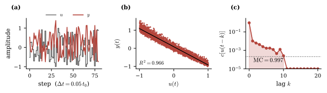
Figure 6. Single visco-piezoelectric fiber read through one electrode. (a) i.i.d. drive and the open-circuit response of the model; (b) scatter plot of vs. with fit recovering of the readout variance; (c) measured forgetting curve , with empirical null marked (gray dotted line).
The readout is very nearly a scaled copy of the input: a linear regression of on the instantaneous drive recovers of the readout variance at a fitted slope of -1 [Fig. 6(b)], so the model is essentially an inverting amplifier. The estimate of the capacity allocated to linear memory nearly saturates the budget, and nearly all of it sits at zero lag [Fig. 6(c)]. In hindsight, this is unsurprising. The model is based on a weakly nonlinear expansion, so its quadratic terms enter the output at in amplitude. Capacity is a fraction of recovered variance, so these contribute only at second order. Appreciable nonlinear capacity would require or of order unity, where the truncation of and the domain condition on Eq. (48) both fail. The concentration at zero lag has a different origin, arising from the dominance of the instantaneous strain’s contribution to the open-circuit voltage over the weaker internal-mode contribution (46).
A physical system realizing these dynamics, embedded in the synthetic skin and capsule of §2.5, may perform useful pre-processing and transduction for a downstream discriminator (perhaps even providing the input to a conventional digital echo-state network in a silicon central nervous system). This is a legitimate device target, but it is not a reservoir. Given that I did not construct the model as a candidate reservoir in the first place, finding that it fails as one is not much of a discovery, and each cause of the failure is a modeling choice, so the result says little about what any given protein fiber system can compute. Raising with more observables, carrying the model past weak nonlinearity, and matching the drive to the relaxation spectrum are the key steps toward a more appropriate model; suggested extensions are discussed in §3.6. Measuring and improving the information-processing capacity of such models, in conjunction with real material prototyping, is a strong target for future work.
3.5Known & unknown challenges
The field remains, in many ways, pre-paradigmatic. The universality results of §3.2 are existence proofs, so they neither guide the construction of a reservoir for a given task nor predict the capacity a specific substrate will deliver. Current hardware optimization proceeds in practice by trial and error.86 Task-independent metrics correlate imperfectly with task performance, and matching a reservoir to a task remains an open problem.110, 121
That physical reservoir computing works across a range of substrates is well established. Whether it is the best way to perform any particular computation is far less clear. After two decades, “broadly convincing ‘killer-applications’ beyond synthetic and lab experiments are still not available,” and reservoir computing performs markedly better on synthetic chaotic sequences than on real-world series such as weather, stock and wind-power data.122 Nonlinear vector autoregression is provably equivalent to a linear reservoir read by a polynomial function, and Gauthier and co-workers report that fitting the autoregression directly matches or exceeds a conventional reservoir on standard benchmarks at a fraction of the cost.102 Those benchmarks are noise-free digital simulations of low-dimensional chaotic systems, so they do not necessarily hold in general. It has also been observed that software reservoirs typically outperform their physical counterparts under comparable configurations, the difference attributed to hardware noise, though exceptions arise where the richer dynamics of a physical substrate happen to suit the task.86 Neither finding rules out a particular physical reservoir winning on accuracy for a particular task, but together they suggest that accuracy may not be the best claim on which to rest a development program.
The stronger case in favor of reservoir computing concerns energy and latency. A passive substrate computes with its own relaxation dynamics at no marginal energy cost per use, and co-locating sensing with computing means the nonlinear, history-dependent part of the transformation is performed where the signal arrives. Only the readout, a set of observables already carrying the computational output in linearly separable form, needs to be transmitted and processed elsewhere. Nonetheless, the advantage is largely unrealized at present. Existing physical reservoirs rely on conventional electronics for input encoding, readout, and environmental control, potentially undermining claims to lower energy use.85, 122 In nearly all reported work, the substrate is a laboratory instrument wired to a computer that records the state and performs the readout regression offline. A device in which the reservoir and its trained readout are built as one has been demonstrated only in memristive electronics,86 and nothing comparable exists for soft, mechanical, or wet substrates.
Reading a soft, spatially extended substrate like a protein-fiber mat is also intrinsically difficult. Probing with tens to thousands of contacts interfaced to analog-to-digital converters is often infeasible on sampling-bandwidth and storage grounds,122 while the observables collected from a continuous medium are strongly correlated, so the usable budget is (§3.3.1).
Stability is a further concern. Hardware drift requires calibration to be repeated, so training cannot be treated as a one-off optimization.122 Soft materials drift with temperature, humidity and light exposure, and can be difficult to characterize even when stable.123 Physical substrates also rarely meet the device-to-device uniformity expected of conventional hardware,109, 119 the disorder that supplies rich dynamics being the same disorder that resists replication.
Readout integration, drift compensation and electrode economy are engineering problems: open, but perhaps tractable. Identifying the tasks and settings in which a physical reservoir beats the alternatives is a different, and perhaps harder question. Protein-based systems may offer rich dynamics and tunable relaxation timescales, but their suitability to the most ambitious visions of this project is by no means settled.
3.6Outlook
No protein fiber device has yet been operated as a physical reservoir. The nearest analogous systems studied for reservoir computing applications are synthetic: a conductive electrospun polyamide mat contacted at several terminals used to drive a simulated reservoir,124 and the nylon fiber networks of §3.4.1.105 The framing of §1.1 placed transduction and computation on one axis, determined by the richness of the I/O map , or by the size of the problem space for which the AR diagram (Fig. 1) commutes. Here, design targets for future work on protein-fiber-based PRC are laid out similarly, ordered roughly by how much computational labor is performed by the material itself.
Instantaneous pre-processing. The material transforms the input signal to support a simple downstream reader’s recovery of the relevant information. This is the role played by the corpuscle model of §2.5: a fixed, passive, untrained front-end that delivers the texture band to the transducer while suppressing the non-information-bearing content of the forcing. Kondo and co-workers demonstrate this in a nonlinear setting: a curved sensor stage encodes softness and pressure jointly, and a simulated ESN downstream does the computing.125 The sensor platform plays the role of a mechanoreceptor, and the ESN is the central nervous system.
Temporal reservoir sensing. Fading memory extends the transformation over a time window to discriminate temporal inputs with only a downstream perceptron. This is where the texture problem of §2.5 was left: the scanning-speed ambiguity of Fig. 5 cannot be resolved from an instantaneous reading. Whisker-inspired sensors designed for real-time terrain classification are one realization of this target.126 A stronger demonstration would reproduce a prescribed nonlinear functional to a stated tolerance. Perhaps the nearest mechanical precedent from the literature is a single nonlinear beam coupled to a delay line, which computed the a parity function of past inputs, though it still relied substantially on external electronics.101
Closed-loop operation. In the targets above, the signal passes through the material once. Closing the loop returns the output as a drive on the same material, so that sensing, computation and actuation occur in one device whose own response becomes part of its input. This is the material as both mechanism and controller. Soft-bodied and tensegrity reservoirs come nearest,94, 127 though error and convergence guarantees for reservoir-based controllers remain unresolved,122 in part because the properties that make a reservoir trainable are established for open-loop driving and do not necessarily survive feedback.
I offer one further target, more as a speculation than as a proposal. Under the material drift discussed in §3.5, a trained readout will continue to confidently report ever-less-accurate outputs. This is awkward, because recalibration against a laboratory reference may be impractical after deployment. But consider human sensing: we too undergo some ‘material drift’ over time, and having a multitude of sensor inputs (backed, of course, by a complex central nervous system) is a great advantage. One input may correct for the failure of another. Standing on one leg is easy until your eyes are closed, and a conversation in a noisy room becomes more intelligible when the speaker’s mouth is visible. Calluses may thicken and alter the mechanical properties of the fingertip, but we scarcely expect to become confused about what we are touching so long as our other senses remain operational. Suppose then that several devices observe the same signal, not necessarily by the same mechanism. Systematic and growing disagreement would identify the drifting unit, and the consensus of the remainder would give a target against which the drifting unit’s readout could be retrained. There is some precedent for this idea in blind calibration of sensors,128 and separately, ensemble averaging over parallel copies of a reservoir driven by a common input has been shown to remove noise and temporal fluctuations from the observed state, restoring (and at times exceeding) noise-free performance.129 To my knowledge, these ideas have not been combined for continual recalibration of an ensemble of drifting physical reservoirs.
One obvious direction for future work is to extend the model constructed in §6.1 and Appendix C to describe a large number of encapsulated transducers in synthetic skin, perhaps modeled on the variety of mechanoreceptors in humans. The model as constructed cannot address such a device. What is required is a spatially-extended continuum through which disturbances propagate. Built this way, the electrode integrals of Eq. (24) could be evaluated on a real strain field, making the instrument profile a design variable to be analyzed systematically against information-processing capacity. This survey did not find any published report combining the required elements. Treatments of coupled compliant networks as reservoirs are well-developed but read displacement directly,98, 105, 116 while continuum models of mechanotransduction in skin resolve the strain field at the receptor but have never been analyzed for capacity.130–131 What the information-processing capacity of such a model would turn out to be is an open and, to my mind, rather appealing question. The original ‘design’, at any rate, works well enough for humans.
4Appendix A: One-dimensional visco-piezoelectric model
4.1Thermodynamic foundations
In this appendix, I derive the one-dimensional visco-piezoelectric model of Sec. 2.1.1. Following work by Coleman and coworkers on the thermodynamics of materials with memory,132–133 define the free enthalpy density of the fiber, whose value at time depends on the entire strain and field histories:
One can show that the dissipation contains terms proportional to and , both free variables, with coefficients and . Were either coefficient nonzero, a protocol to perform some net work with zero dissipation could be selected, so thermodynamic consistency requires both to vanish identically. This yields132
Here the derivatives are taken with respect to the present values of and .
The non-Markovianity (history dependence) of the free enthalpy in the strain and electric field indicates the presence of hidden variables. Introduce an internal state vector such that the free enthalpy is Markov in .134 These do not need to exhaust all of the system’s degrees of freedom, only the slow internal rearrangements (e.g., ionic redistributions). Take to be the rest state and set (WLOG) . Taylor expanding about its rest state and retaining up to cubic terms that are at most linear in and yields
From this, obtain by differentiation [Eq. (38)]
The linear terms in and in (40) reproduce the standard constitutive equations of piezoelectricity with , , and respectively the high-frequency limits of the elastic modulus, piezoelectric coupling, and permittivity at the rest state. These terms characterize the instantaneous response at fixed .
In line (39), the term is the leading elastic anharmonicity, producing a stiffness that grows with strain, as observed in compressed collagen.53–54 The term is a nonlinear coupling between the field and the strain. The cubics and in have been excluded since in open-circuit sensing, the field is generated by the strain, so it is itself first-order small.
Since the internal state vector is not directly observable, its coordinates may be chosen freely. It is convenient to take them to be normal modes, which simultaneously diagonalize friction and stiffness so that no cross-terms enter. Each mode then relaxes at first order,
with time constants set by friction coefficient and stiffness . A finite collection of modes produces a discrete relaxation spectrum, which is commonly assumed in viscoelastic modeling, if not perfectly general.52 As a sanity check, the entropy production under these dynamics is .132 The weights and determine the response of mode to strain and field, and the cross-terms in (41) and in (40) (from the cubic ) represent strain-stiffening via the relaxation modes. I have excluded cubics that are nonlinear in purely for the purposes of tractability, as retaining those terms would make the relaxation times themselves dependent on the drive amplitude.
4.2Non-dimensionalization
Let be a characteristic amplitude of the driving strain. Then we have natural scales for the field, for internal mode , and and for stress and displacement. The linear response of the system is then characterized by four families of dimensionless numbers,
The first is the electromechanical coupling factor, or the fraction of elastically stored energy available for conversion to electrical form, with required for stability. (resp. ) is the fraction of the elastic modulus (resp. the piezoelectric coupling) removed by mode as it relaxes. Note that necessarily, while may take either sign, as observed in ferroelectric polymers.61 Finally, is the relaxation time of mode measured in units of the slowest relaxation time, .
The nonlinearities contribute three further groups of dimensionless numbers,
respectively the fractional stiffening of the modulus, the ratio of quadratic to linear charge, and the ratio of quadratic to linear drive of mode , all evaluated at the drive amplitude . Each scales linearly with , and the input amplitude enters only through these numbers. Thus the model is “weakly nonlinear” if . In total, the model comprises numbers: together with for each mode.
In a blatant abuse of notation, let us rescale every variable while retaining the original symbols, taking all variables dimensionless henceforth:
For the rest state to be stable, we require
These conditions bound the admissible parameter space.
4.3Open-circuit reduction
Reading the fiber into a high-impedance amplifier imposes the open-circuit condition , giving
exactly the voltage measured in units for fiber length . This serves as the model’s output. Substituting this back into the model yields
Note first that the linear stiffness is , recovering exactly the standard open-circuit piezoelectric stiffening of the modulus.64 Second, the internal modes are now effectively coupled, since each mode’s charge contributes to the shared field, which in turn drives all modes.
The strain appears now only as an auxiliary quantity, fixed at each instant by the balance between the applied stress and the stress sustained by the material. That balance is set by Eq. (47), a quadratic in . The physical root is the one that reduces to the linear solution (for total linear drive and state-dependent stiffness , defined in Eq. (49)) when the quadratic stiffness vanishes:
Here we have passed to the notation of the I/O map (4): the input is the applied stress, , the internal state is the mode vector, , the output is the field, , and is the strain the fiber adopts under stress with its internal state at . With every constant coefficient reduced to a single symbol (Table 2), the model is
The square root in Eq. (48) delimits the model’s domain: if the drive is strong enough that , the weakly nonlinear description has been pushed past its regime of validity. In simulations this condition is monitored and treated as a bound on the admissible drive amplitude.
Symbol | Definition | Meaning |
open-circuit (stiffened) modulus | ||
total instantaneous quadratic stiffness | ||
square-law charge coefficient in the readout | ||
open-circuit relaxation strength of mode | ||
charge carried per unit displacement of mode | ||
strain–state cross stiffness | ||
field-mediated feedback of mode | ||
linear drive of mode | ||
quadratic drive of mode | ||
relaxation timescale matrix |
5Appendix B: Survey of transduction mechanisms
This appendix expands §2.2, characterizing each mechanism by its material coupling coefficients and their microscopic origins. The survey is not comprehensive, the relative space given to different mechanisms is best regarded as a reflection of time and attention constraints, rather than as a reflection of their relative promise.
5.1Dielectric couplings
Electromechanical couplings, and in particular those found in dielectrics, are well-supported at both the level of bulk systems40, 120, 135 and individual fibers.36, 136 A dielectric material is characterized by low conductivity and the induction of a polarization in the presence of an external electric field .
It may be instructive to see how a family of couplings can be unified within a single thermodynamic scaffold. Let be the Gibbs free energy of an elastic dielectric for temperature , stress , and applied electric field . The extensive conjugates to and are the entropy , strain field , and electric displacement vector , and their total differentials reveal a collection of couplings64:
The piezoelectric and pyroelectric phenomena emerge cleanly as off-diagonal terms of Eqs. (51) and (51). I discuss these in more detail below, and then introduce flexoelectricity, the generation of electric polarization by a strain gradient, and ferroelectricity, characterized by a bistability in the polarization vector.
5.1.1Piezoelectricity
Piezoelectricity is the direct conversion between mechanical strain and polarization , and occurs in all non-centrosymmetric dielectrics. Synthetic piezoelectrics are ubiquitous, from electronics to biomedicine, but are often rigid or toxic, limiting their use in some applications. Piezoelectricity has significant experimental and theoretical support in proteins, and biocompatible piezoelectric devices are an active area of research.14, 30, 32, 60, 135, 137–140 The central engineering challenge is their relatively weak response and the poor scalability of current manufacturing.45
Piezoelectricity is usually characterized by the piezoelectric coefficients
a third-rank tensor (see Eqs. (51), (51)) reported in or, equivalently, . In the linear regime (small fields/strain) these are treated as material constants, but the coupling is nonlinear in general (e.g. electrostriction is the second-order coupling 64).
Atomistic simulation reveals how applied stress reorients and rescales the permanent dipoles of individual charged and polar residues, producing a net polarization along the fiber axis.27 Because this polarization is axial, parallel fibrils add while antiparallel ones cancel. Piezoelectricity in bulk tendon therefore reads roughly an order of magnitude below a single fibril, whose contribution is diluted in tissue by oppositely oriented neighbors.36 This is the basis of the alignment result stated in §2.2. Crosslinking-driven self-assembly to enhance piezoresponse has been reported in the literature.34
Reported magnitudes span a wide range: e.g. collagen fibrils and films at ,45 self-assembled diphenylalanine peptide nanotubes reaching with a linear and fully reversible response up to ,136 against inorganic PZT’s .43 Note, however, that these numbers as stated are not easily comparable, differing in tensor component (, , , … in Voigt notation), measurement protocol, and length scale.60
The tensor component matters greatly, with shear coefficients typically dominant over the axial coefficient in chiral polymers, including in collagen and self-assembled diphenylalanine peptide nanotubes.44, 57, 59 A fiber loaded in pure tension is therefore driven through its weakest coefficient. The stronger shear response could be reached by converting axial drive into torsion, or by electrodes arranged to collect shear-generated polarization, and it offers a further advantage in being less sensitive to the disorder that cancels the axial response. The challenge is in designing an architecture that realizes this at device scale.
5.1.2Pyroelectricity
Pyroelectricity is the change in the spontaneous polarization in polar materials in response to a change in temperature. Theory often takes the pyroelectric coefficient as the fixed-field temperature dependence of : , but the relevant quantity is more often the generalized coefficient (via ) which captures pyroelectric-like responses that arise even in non-polar dielectrics under an electric bias. The coefficient of Eq. (51) is the ‘free’ coefficient, since fixed stress lets the material expand thermally.
Strong piezoelectricity enhances pyroelectricity.64–65, 141 The ‘clamped’ coefficient at fixed strain is the primary response alone, while the ‘free’ coefficient at fixed stress includes charge from thermal expansion and piezoelectricity (the secondary contribution):
where is the elasticity tensor and is the thermal expansion tensor.
5.1.3Flexoelectricity
Flexoelectricity is the generation of polarization by a strain gradient (direct effect), or of strain by a field gradient (converse effect).142 With material coordinates , piezoelectricity and flexoelectricity are the first two terms in the gradient expansion of the electric displacement:
where . The flexoelectric response is the fourth-rank polar tensor , which is nonzero even in centrosymmetric materials where identically. This makes it more general than piezoelectricity, if less well understood.
Its chief limitation is scale. The extra spatial derivative carries an inverse length, so the effect scales as : negligible in bulk but potentially competitive with piezoelectricity at the nanoscale,142 hence of particular interest for individual fibrils, though to my knowledge no flexoelectric coefficient has yet been reported in an individual protein fibril. It has been proposed as a key coupling in hearing, poising the cochlear hair bundle at a Hopf bifurcation so that faint sounds trigger large, self-sustaining oscillations.143 The soft-matter theory of flexoelectricity remains immature, however.144
5.1.4Ferroelectricity
A ferroelectric is a pyroelectric whose spontaneous polarization has two or more orientations, interconvertible by an applied field. The phenomenon is native to proteins. Ferroelectric switching was first uncovered in porcine aortic wall by piezoresponse force microscopy,145 and subsequently localized to its elastin. Switching of a purified elastic fiber network under an applied field was shown both at the nanoscale and macroscopically.146 Collagen, run as a control in the same experiment, does not switch. Switching in aortic elastin is also suppressed by glucose,147 a liability for an implanted device but perhaps an exploitable chemo-ferroelectric coupling.
Beyond fibers, ferroelectric switching has been resolved in crystalline -glycine,148 whose polymorph carries the large shear piezoelectric response discussed in §5.1.1.32 Bistability suits a ferroelectric to memory or logic rather than to pure transduction, and a retained, switchable state is a different computational resource from the fading memory Ch. 3 relies on. This document does not explore that possibility, though it may be of interest for future research.
5.2Triboelectricity
Triboelectricity is the transfer of charge between two materials brought into contact or slid against one another (everyday static electricity being its most familiar form). It is an electromechanical coupling, but qualitatively distinct from those above. It is interfacial, depending on a pair of surfaces and their contact history, so there is no material-level constitutive relation. The mechanism is itself unsettled (whether the transferred species are electrons, ions, or both is debated and differs between material pairs) so characterization is necessarily device-level and phenomenological.
There is a well-developed literature on exploiting triboelectricity in devices. This is particularly true for energy harvesting, with a large body of work on triboelectric nanogenerators (TENGs). Electrospun fiber mats are attractive substrates because their high surface-to-volume ratio maximizes the interfacial area over which charge transfers; see Ref.149 for a recent review, including how coupled solution and process parameters set fiber morphology (and hence output).
5.3Electric and ionic transport
The conductivity of a material is
where and are respectively the majority carrier’s charge, number density, and mobility. The interesting physics lives in and and their interdependence, set by the localization of conducting states, structural and energetic disorder, and the carrier’s coupling to its local environment.58
The majority charge carrier may be an electron, a proton, or a larger ion, with biological precedent for each. Neuronal and cardiac signaling involve , , and fluxes, and transmembrane proton () transport drives mitochondrial ATP synthesis.58 Long-range electron conduction along protein nanowires has drawn considerable attention recently, in the nickel-cofactor wires of cable bacteria150 and the conductive micrometer-long polymers of the cytochrome OmcS in Geobacter.151–152
Conduction theory is mature for crystalline inorganics, far less so for disordered biomolecular systems. Isolating the current-carrying physics is hard, with mechanisms and carriers routinely conflated. Measuring ion transport is much more difficult than measuring electron transport, partly because standard metal electrodes simply block protons or ions. Melanin is the cautionary tale: long modeled as an electronic (Anderson-hopping) semiconductor, it is now understood to conduct predominantly by protons.58 Whether a conductor is proton- or electron-dominated can be tested by comparing conductivity in versus (a kinetic isotope effect experiment11).
5.3.1Ionic and protonic conduction
Ionic conductors have matured over more than half a century, and the proton-conducting polymer Nafion is now used in commercially available fuel-cell membranes.58 The two main mechanisms are purely diffusive transport ( for diffusion coefficient and thermal energy ) and the Grotthuss mechanism, the rapid relay of an ionic defect through a hydrogen-bonded network. The latter is typically much faster and depends on the ordering and polarization of the participating water molecules. A percolation-like transition between the two regimes with a power-law dependence of conductivity on hydration near the transition has been suggested, but not verified.
Protonic conduction has been realized in designed protein fibers. A self-assembling tripeptide (Lys-Tyr-Tyr) forms melanin-like films conducting up to at relative humidity,11 and prion-inspired amyloid fibers built on an X–Tyr motif reach at 40C, rising to at 120C.29 In metalloprotein nanowires, it has been reported that carboxylic-acid groups are the essential functional groups, increasing the number of proton-transfer pathways when hydrated.28 This points to aspartate- and glutamate-rich sequences as a rational design lever.
In all cases ionic conductivity rises steeply with hydration (in collagen, by several orders of magnitude from dry to saturated) and is strongly temperature-activated. It is commonly raised by adding protonatable sites for Grotthuss-type hopping and hydrophilic moieties for water uptake. In chitosan films, greater chemical crosslinking reduced crystallinity and so increased the conducting amorphous fraction.58
5.3.2Electronic conduction
Where electrons carry the current, the operative mechanism in protein fibers is redox hopping between closely spaced cofactors or aromatic residues. Microbial “nanowires” are micrometer-long polymers of the cytochrome OmcS, whose closely stacked hemes provide a continuous path for electron flow.152 The periplasmic wires of cable bacteria carry electrons over comparable distances through a protein core built around a nickel cofactor.150 In engineered peptide- and protein-based structures, the high reported conductivities usually come from a conductive coating (PEDOT:PSS, polypyrrole, or polyaniline), with the protein serving as a mechanical and morphological scaffold.58, 153
5.3.3Piezoresistance
Piezoresistance is the modulation of conductance by mechanical strain. It is grouped here as it modulates a transport coefficient rather than generating a polarization, so it needs an external read current. A material of resistivity , length along the transport axis, and orthogonal cross-section has resistance . Deformation may alter any of the three parameters. As with the electronic conductors above, piezoresistance in protein-fiber systems is typically a property of an added conductive phase like carbon nanotubes, silver nanowires, or a conducting-polymer coating.58, 66, 153
5.4Capacitive transduction
A capacitive element transduces deformation into a change of capacitance. For a parallel-plate idealization , deformation changes the electrode area , the separation , and (for a strained dielectric fiber) the permittivity itself. Capacitive sensing reports static deformation at the cost of an excitation signal and a sensitivity to stray capacitance.
Ionotronic designs, in which an electric double layer forms at an electrolyte–electrode interface, confine the field to a nanometre-scale region and so reach capacitances unattainable with conventional dielectrics, giving sizable low-voltage signals compatible with wet protein systems.67–68 Moreover, the sensitivity can be tuned geometrically. For example, cricket-inspired MEMS hair-flow sensors read the deflection of a high-aspect-ratio pillar through a differential capacitance.154 See Refs.155–156 for a survey of hair-sensor designs and for a critical comparison of the impedance and dielectric spectroscopy methods used to characterize these interfaces.
5.5Light-coupled mechanisms
Light may be the transduced output of a mechanical or electrical input, or the input driving a mechanical or electrical response. All four mechanisms below have been demonstrated in electrospun or self-assembled fibers.
5.5.1Mechanoluminescence
Mechanoluminescence converts mechanical energy directly into light, and piezoelectricity can enhance the response. The canonical emitter is manganese-doped zinc sulfide (), which has been integrated into electrospun PVDF-based nanofibers.42 There the emitted intensity varies linearly with applied pressure over the tested range and nonlinearly with membrane thickness. Efficient, sensitive mechanoluminescence remains an open engineering challenge.157–158
5.5.2Electroluminescence
Electroluminescence is light emission driven by an applied field. A representative realization is the “scalable hydrogel-clad, ionotronic, nickel-core electroluminescent” (SHINE) fiber,16 in which microparticles dispersed in a dielectric are sandwiched between a nickel core and a hydrogel cladding to form a capacitor. It sustains a luminance of under a AC field.
5.5.3Photomechanical actuation
Photomechanical actuation is deformation in response to illumination, typically through a photoisomerizing moiety. Azobenzene is the standard example, switching reversibly between trans and cis isomers under different wavelengths. The accompanying conformational change can drive bulk motion: azobenzene has been incorporated into protein fibers for light-induced, reversible modulation of stiffness,159–160 and electrospun azobenzene/cellulose fabrics bend toward a UV source.161 The reported effects are slow and the strains modest, which confines the mechanism to applications tolerant of subtle motion, perhaps with geometric amplification.
5.5.4Photoconductivity
Photoconductive transduction converts incident light into an electrical signal by generating free carriers in a semiconductor. In fiber form it has been realized by electrospinning or coating a semiconductor, such as a metal oxide or a halide perovskite, into a single fiber or mat. Individual electrospun fibers reach responsivity in the UV,162 and PAN/ composite fibers extend the response into the visible range.163
5.6Others
The mechanisms above do not exhaust the map of Fig. 2. Several additional couplings are interesting as input or output stages, and are noted briefly:
Thermoelectric (steady temperature gradient voltage, the Seebeck effect). Fiber-compatible conducting polymers such as PEDOT:PSS may suggest a route to thermoelectric fibers,164 adding a fifth harvesting modality alongside piezo-, pyro-, tribo-, and photovoltaic.
Thermo-mechanical (temperature or confinement shape change). Silk fibroin confined in a carbon-nanotube sponge acquires a shape-memory effect.165
Hygroelectric (moisture gradient charge). Protein nanowires can generate sustained power from ambient humidity alone, with no mechanical input.166 The hydration dependence that complicates ionic conduction here becomes a source of energy.
Chemo-mechanical / chemo-electrical couplings, in which ligand binding or a change in solvent drives swelling, conformational change, or a shift in charge state. Aligned electrospun silk fibroin bundles infused with conducting polymers actuate electromechanically in biologically relevant electrolytes at low applied potential,15 and organic electrochemical transistors transduce biomolecule binding into a current.71
Structural phase transitions (stress large-scale structural change). Predicted for collagen fibrils167 and observed in first-order form,168 these couple stress to structure with a gain that diverges near the transition. They receive no further consideration in this document, a notable gap that reflects limited time rather than limited promise.
6Appendix C: Case study: Mathematical details
6.1Loewenstein-Skalak model
This appendix analyzes the lumped Loewenstein–Skalak (LS) model of the Pacinian corpuscle introduced in §2.5.2 [Fig. 4(b)].78
Index the lamellae from innermost to outermost, and let denote the displacement of lamella along the loading axis. Each lamella is an elastic membrane of stiffness , drawn in Fig. 4(b) as a spring to the rigid frame. Between lamellae and sits a viscoelastic fluid layer mostly composed of water and collagen, modeled as a Kelvin–Voigt element with spring constant and viscosity . The innermost layer couples lamella 1 to the core and is taken to be rigid (). The external force enters at the outermost lamella, . Neglecting lamellar inertia and defining the complex inter-layer stiffness , the force balance on lamella reads, in the frequency domain,
with boundary conditions and .
The force at the core is the stress transmitted through the innermost fluid layer, so the transfer function of the capsule is
The equations of motion (56) form a tri-diagonal system
where is the th Cartesian unit vector, so . For a tri-diagonal matrix the corner element of the inverse collapses: the cofactor is a triangular minor whose diagonal holds the superdiagonal entries , whence and
This reads as the impedance of the final fluid layer times the complex admittance carrying mechanical signals from layer to layer 1.
The essential behaviour is already present for a single layer (), where
Following Loewenstein & Skalak, take , i.e., the inter-lamellar couplings are far more compliant than the membranes themselves. Three regimes follow at once:
: static forces produce almost no force on the core.
: signal strength grows linearly in .
: near-perfect transmission of high frequencies.
The zero at and pole at bracket a differentiating band in which the capsule reports the rate of loading, and the exact DC transmission is .
For the full model as , i.e. each coupling acts as a spring under static loads. For identical layers (, ), Eq. (59) gives , where is the th continuant of the tri-diagonal coupling matrix :
By careful substitution, one finds that
Static transmission falls off geometrically with depth, with each fluid layer passing only the fraction of its outer neighbour’s displacement inward.
In the limit , the dashpots rigidify and the stack translates as a rigid body, and the load is transmitted to the core in full (). The radially graded parameters estimated by Loewenstein & Skalak from empirical data improve the static suppression even further.78
6.2The embedded capsule
When the capsule is embedded in a skin (§2.5.3), the primary input variable under the external drive is the displacement of the skin patch, and the system gains an extra node beyond the LS model. Model the skin patch as an inertial spring-damper system with impedance
coupled to the outermost lamella by the tissue element . The force balance on the interior lamellae is unchanged from Eq. (56), but lamella now couples outward through :
In the frequency domain, Newton’s law for the skin patch reads
Write , so , with identical to in rows and
The total transfer function is now
still read intuitively: the transfer of the external drive to the internal force is given by the skin’s elastic coupling times the complex admittance from the capsule’s core to the skin times the impedance of the innermost layer of the capsule . This can be decomposed further in a physically meaningful way.
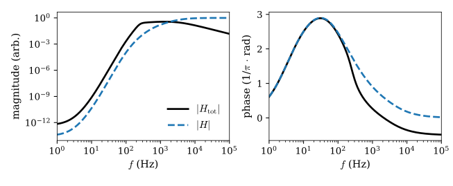
Figure 7. Transfer functions of a capsule with layers, uniform stiffness contrast , and relaxation frequencies graded logarithmically over 2–60 Hz from exterior to interior. For the skin patch, N/m, g, and N s/m, coupled through a soft tissue element N/m. Skin patch values were selected to be similar to the measured mechanical behavior of a fingertip.75 (a) Magnitude of the bare-capsule response (13) (blue, dashed) and the total embedded response (70) (black, solid) in arbitrary units. (b) Unwrapped phase in units of . The peak of indicates roughly six layers of simultaneous differentiation, consistent with the slope on the rising flank in (a).
Define the input stiffness , the ratio of applied force to the displacement of the driven lamella. The skin patch sees the series combination of the tissue element and the capsule:
Expanding along its final row in the continuants (61) of the bare capsule yields
and so using [Eq. (59)] the transfer function factorizes as
where is the transfer function of the capsule. The factor accounts for the back-reaction of the capsule on the skin. When (i.e. the receptor is far more compliant than the skin patch), the capsule reads the local skin motion without meaningfully deforming it.
At , the skin gain is , so the static suppression remains geometric in depth (62), with one extra spring divider. For , the inertial term dominates and , curing the nonphysical flat tail of Eq. (60). See Fig. 7(a).
Footnotes
Pancomputationalism is essentially the view that every physical process is a computation. This renders the notion rather vacuous, especially if one is trying to actually build a physical computer.169
↩Here gives the domain and codomain (input and output spaces) of a map, and gives its action on one element.
↩The identification of with the input coupling will typically be far more subtle than stated here. For instance, the task of the computer might be to process a continuous stream of information at the inputs, with reflecting both present and past signals. In that same situation, is not merely the autonomous evolution of from its initial instantiation but rather a functional of both the initial conditions and the input history.
↩The macrostates representing bits in a digital machine, for instance.
↩For instance, the system is assumed to operate at equilibrium. The analysis in a driven system may be very different.
↩Though it is in principle possible to either falsify the form or fix the coefficients with experimental measurements of a real visco-piezoelectric fibril. See, e.g., Ref.170.
↩Bulk tendon reads roughly an order of magnitude below a single collagen fibril for this very reason.36
↩The derivation is brief: Since no free charge flows in open circuit, . Thus any induced polarization must be canceled by an internal field .
↩Permittivity measures how much of an applied field a material absorbs into the rearrangement of its own charges. In a high-permittivity material, internal rearrangements in response to a stress-induced field leave little for an electrode to measure. A low-permittivity material leaves that charge exposed, and the voltage is correspondingly larger.
↩In more detail: (§5.1.3), which I take to be proportional to the bound fraction for simplicity. From the Hill equation with Hill coefficient 1, gives .
↩Psychophysically, texture is a small handful of weakly related perceptual axes (shine/matte, coarse/fine, rough/smooth, sticky/smooth, and so forth).72, 171 Its definition is much more complicated than acknowledged here, as “there is little agreement as to what constitutes texture”, and “the definition will vary with the sensory system that transduces the surface”.72
↩Natural surfaces are often approximately self-affine within some finite band of wavenumbers , with the lower limit corresponding to a wavelength –m for many engineered surfaces81. The spectrum obeys a power law in this regime, with Hurst exponent .74, 81 At fixed large-scale amplitude, small places relatively more power in fine features.
↩These ranges are similar to those cited in human perception studies (e.g. Manfredi et al. present textures at 4–12 cm/s82), but are deliberately wider, since a synthetic skin need not be confined to the kinematics of human touch.
↩The LS model was developed in 1966, and though it remains an elegant demonstration of a plausible mechanical filtering mechanism, it has long been recognized as overly simplistic,77 and recent research may overturn this picture of frequency selectivity entirely.172 The case study’s engineering value does not depend on the biology being right, and indeed, it should by no means be regarded as a model of how texture perception actually works in vivo.
↩A restrictive and likely unrealistic assumption, to be sure.
↩Intuitively, the recent past is weighted more heavily in the output than the distant past. Fading memory is defined more carefully in §3.2.3.
↩These include Nakajima’s introductory perspective on physical reservoir computing,85 and the edited volume of Nakajima and Fischer, Reservoir Computing: Theory, Physical Implementations, and Applications.5 Another worthwhile resource is the hands-on Jupyter-notebook-based tutorial of Cucchi et al.109
↩Conventionally this is the hyperbolic tangent , whose saturation both supplies the nonlinearity and keeps the state bounded.
↩This model is not totally general, and many conventional features can be relaxed. For instance, the weights and needn’t be random. A deterministic cyclic network with a single connection weight is competitive with a fully random ESN across standard benchmarks, with reservoir size rather than structural complexity carrying performance.173
↩Stated in this way, the property seems to exclude stochastic dynamics, since a noisy state is not a function of the input history alone. The strict form is not needed. It suffices that trajectories under a common drive converge to within a noise floor, and that floor then bounds what the readout can recover (§3.2.3, §3.3.2).
↩This guards against ill-conditioning of the state Gram matrix and against overfitting the readout to noise. Ordinary least squares is recovered for .
↩See, e.g., the chapter by Dale et al. in Ref.5, adapting Konkoli et al.
↩Boyd’s result is stated for inputs with finitely many temporal channels, , so one should restrict to , decomposable over a finite set of fixed spatial profiles. The profiles might correspond to instrument profiles of separate actuators, contacts, or electrodes.
↩As noted above, FM is equivalent to Jaeger’s echo state property, and the same property is sometimes called common-signal-induced synchronization107 or consistency,174 mostly depending on the academic background of the authors.
↩The echo state property can be generalized to an echo index that counts the number of coexisting driven responses in a system for a particular subset of inputs, and a reservoir must have an index of one over its operating regime.175
↩This was introduced by Jaeger before the general information capacity was defined.88
↩See, for example, the spontaneous conductance relaxation and paired-pulse response of self-organized nanowire networks 92 or the conductance recovery of liquid albumen.95
↩See, e.g. Eq. (40): gives for .
↩Note that neither source covers the case at hand directly. Coleman (1964)132 treats deformable media with memory but no electromagnetism; Coleman & Dill (1971)133 treat electromagnetic fields in materials with memory but confine themselves to stationary media to avoid the difficulties arising from the interaction between material motion and the field. The model here borrows the form of their arguments without establishing that the procedure remains valid for the coupled electromechanical case.
↩The substitution also generates a term , a product of two first-order-small nonlinearities. It lies beyond the truncation order of and is dropped for consistency.
↩By convention, applied stress induced charge density is direct piezoelectricity and applied field induced strain is converse piezoelectricity. Here, I do not disambiguate, and refer to both directions as “piezoelectricity”.
↩The permittivity carries the same boundary-condition ambiguity. and differ by as much as 50-,64 and the right choice depends on the device’s operating regime.
↩The cis isomer also relaxes thermally, though relatively slowly.
↩Since , this transfer function is nonphysical,176 so it is best read as a simplified approximation of the true transfer function over a finite band.
↩
Be the first to comment on this publication.