Purpose
Arcadia looks beyond the standard model organisms for systems that can teach us about biology. Zoogle, Arcadia's phylogenetics-informed organism selection tool, identified the green alga Chlorella vulgaris as a strong candidate. Thousands of its proteins, spanning many different pathways and functions, are more similar to their human counterparts than evolutionary distance would predict. We used high-throughput imaging to measure dozens of morphological features in 91 UV-mutagenized strains across six growth conditions, determining each feature’s discriminatory power and sensitivity to noise. Most features consistently distinguished strains across fields of view, while others showed little reproducible signal. Together, these measurements allowed us to predict phenotypes in a held-out condition for strains not included in model training. Future screening, knockouts, rescues, and human variant testing will build on this work. We think this approach of establishing tractability before launching large screening campaigns may be broadly useful, and we'd especially appreciate feedback from people working in this area.
Background and goals
Much of biomedical research rests on a short list of model organisms. They earned that status largely through convenience. They grow quickly, they’re easy to keep, and decades of work have built up the genetic tools to manipulate them. But convenience isn’t the same as relevance. Evolution has preserved pieces of human biology in organisms scattered across the tree of life, and for a given question, the best system to study it in may not be one of the usual suspects. At Arcadia, we’re trying to find those organisms systematically, letting evolutionary evidence decide where to look rather than defaulting to what’s familiar.
Zoogle 1–2, one of the phylogenetics-informed tools we’ve built, is one way we do that. When we compared 62 organisms across the 6,322 human genes with a Chlorella homolog in Zoogle, the unicellular green alga Chlorella vulgaris stood out. For 682 of those genes, its homolog ranked first in phylogenetic-distance-corrected similarity to the human protein, and for 1,209 it ranked in the top three. C. vulgaris is already a well-studied, easily cultured microalga 3, so on paper, it’s an appealing platform for perturbation-based studies of conserved cellular processes. But looking good on paper doesn’t make an organism useful in the lab.
For an organism to be useful as an experimental platform, it isn’t enough for its cells to look different from one another 4. Those differences need to be reproducible, they need to shift in response to perturbations in ways we can map, and they need to reflect biology rather than measurement noise. So before investing further in Chlorella, we wanted to know whether its phenotypes clear that bar. Specifically, we asked whether Chlorella mutants show phenotypic variation that’s reproducible, responds to environmental conditions, and follows patterns we can learn and predict.
That raised a practical question: What should we measure? We decided to use microscopy to measure a suite of morphological features at scale without relying on exogenous labels. Chlorella also brings a label of its own. Its large chloroplast is autofluorescent, giving us a built-in readout that’s widely used to track photosynthetic state 5 and should be sensitive to perturbation. If these features turned out to be mostly noise, we’d know Chlorella wasn’t ready to screen with this set of phenotypes. If they held up, we’d have something to build on.
The approach
We used UV mutagenesis to generate a panel of Chlorella vulgaris mutants, grew them under different conditions (three temperatures × two growth stages), and measured how they looked. We imaged cells without labels in two channels: bright-field and Cy5, which captures chlorophyll autofluorescence. An automated pipeline then segmented more than 8.3 million cells across both channels and extracted 40 morphological features. Finally, we asked which features reliably distinguish one strain from another, and we trained a model to predict each strain’s phenotype in one condition from its phenotypes in the other five.
Generation of genotypic diversity
We generated genetic diversity using UV-induced random mutagenesis, which produces a broad range of genotypes and is straightforward to implement. We didn't genotype the resulting strains, though nothing about this approach precludes doing so later.
In brief, we used 10 mL of Chlorella vulgaris strain 211-11P 6 grown in Tris-acetate-phosphate (TAP) medium (ambient light, 22 °C, OD700 = 1) and irradiated it in a 100 mm glass petri dish with UV-C (254 nm) light using a Stratalinker 2400 UV Crosslinker (Stratagene, #400075). To pick an exposure, we ran a UV dose titration and scored colony formation across doses. We chose a dose near the low-survival end of that range, 830 mJ/cm2, reasoning that a heavier mutational load would give us a more phenotypically diverse population to sample. A milder dose would likely have produced viable mutants too, just with fewer lesions per genome and a narrower phenotypic spread. Following irradiation, we incubated cells in the dark for 24 h to inhibit photorepair pathways 7, then seeded them onto TAP plates (TAP medium with 1.5% agar) for colony isolation and viability assessment.
At the dose we selected, viability was roughly 0.5% relative to non-irradiated controls by colony count. Since our aim was to characterize phenotypic diversity across the mutagenized population rather than to link phenotypes to specific mutations, what mattered was that the population carried a broad range of genotypes, not that it hit a particular survival number. From this population, we used sterile toothpicks to isolate 96 randomly chosen mutants into a round-bottom 96-well plate for downstream phenotyping assays. We generated a matched wild-type comparison by following the same protocol without UV exposure, resulting in 96 isolated wild-type clones. UV-derived strains and the wild-type isolates were not intended to be retained indefinitely, and independently generated UV mutants cannot reproduce strain-level results.
Growth and environmental perturbation design
TAP medium: 7.5 mM NH4Cl, 0.34 mM CaCl2·2H2O, 0.41 mM MgSO4·7H2O, 0.62 mM K2HPO4, 0.41 mM KH2PO4, 20 mM Tris base, 17.5 mM glacial acetic acid, and 0.1% v/v Hutner’s trace elements solution in ultrapure water, adjusted to pH 7.4 with NaOH. Final trace element concentrations were 134 µM Na2EDTA·2H2O, 77 µM ZnSO4·7H2O, 184 µM H3BO3, 26 µM MnCl2·4H2O, 18 µM FeSO4·7H2O, 6.8 µM CoCl2·6H2O, 6.3 µM CuSO4·5H2O, and 0.89 µM (NH4)6Mo7O24·4H2O.
We grew cultures in TAP medium in 96-well deep round-bottom plates (VWR, 75870) covered with breathable sealing films (Excel Scientific, #B-100). We maintained them in shaking incubators (200 rpm) to ensure adequate mixing and aeration. We illuminated cultures under a 16 h light/8 h dark cycle with low-intensity (about 800 lux) blue light (460–480 nm) delivered via custom-built light boxes. To initialize the experiment, we split all strains across three plates, one per temperature, keeping each strain in the same well position on every plate, and diluted them to identical seeding densities (OD700 = 1), then diluted 1:20 in 1 mL total TAP medium per well. Because we grew cultures at each temperature on a single plate, effects we attribute to temperature also include plate-level differences.
Download 3D printing files for our custom light box from NIH 3D.
We profiled mutant strains across six environmental conditions, defined by three temperatures and two growth stages. We grew strains at three discrete temperatures (16 °C, 22 °C, and 30 °C), spanning a biologically relevant range 8 that modulates growth rate and cellular physiology. We collected data at two discrete time points, which we refer to as early stationary phase (four days post-seeding) and late stationary phase (10 days post-seeding). We selected these time points to capture transitions and persistence within nutrient-limited conditions, but we didn’t confirm growth phase for each strain and temperature, so strains may differ in growth stage at a given time point.
Imaging and feature extraction
To quantify cellular phenotypes, we performed label-free imaging of mutagenized Chlorella strains and extracted single-cell-level features. We imaged cells using a Yokogawa CSU-W1 SoRa spinning-disk confocal unit mounted on a Nikon Ti2-E inverted microscope, equipped with an ORCA-Fusion BT sCMOS camera (Hamamatsu) and a LIDA Light Engine (Lumencor) for illumination, controlled with NIS-Elements software (RRID: SCR_014329; v6.20.02). We acquired all images with a Plan Apo λ 20× objective (numerical aperture 0.75), yielding an effective pixel size of 0.216 µm. We imaged in two channels: bright-field and Cy5, using 640 nm excitation and collecting emission in the approximately 700 nm band to capture chlorophyll autofluorescence.
We automated acquisition using NIS-Elements JOBS 9 (v6.20.02) to sample each well systematically. For each well, we acquired 25 fields of view and used the first nine for analyses (due to diminishing returns), giving 819 field-level observations per condition (91 strains × 9 fields). Before imaging, we diluted cultures 1:10 in TAP medium (100 µL of cells were aspirated for dilution and replaced with TAP) and transferred 100 µL of diluted cells to glass-bottom plates for appropriate density and optical clarity.
We processed raw images with the help of Arcadia microscopy tools 10 (v0.1.0; RRID: SCR_029206). Segmentation was done by Cellpose-SAM 11–12 (v4.0.7), while feature extraction was done using scikit-image regionprops 13 (v0.25.2). Before segmentation, we corrected for illumination variation across fields of view using background subtraction and percentile-based intensity rescaling 14 (see segmentation details). We visually checked segmentation on representative images from each condition. Across all conditions and channels, we segmented 8,334,079 cells.
Access our microscopy data on BioImage Archive.
Computational notebooks for processing images, segmenting cells, etc. are available in our GitHub repo (DOI: 10.5281/zenodo.24383650).
| Feature | Description |
|---|---|
| count | Number of cells in the field of view. Reflects culture density at the time of imaging. |
| area | Size of the cell in pixels. Reflects the total footprint of the cell body within the imaging plane. |
| area_convex | Size of the smallest convex shape that fully encloses the cell. Cells with irregular or concave boundaries will have a convex area larger than their actual area. |
| perimeter | Length of the cell's outer boundary. Larger or more irregularly shaped cells tend to have longer perimeters. |
| eccentricity | How elongated or circular a cell is. A value of 0 indicates a perfect circle; values approaching 1 indicate increasingly elongated (elliptical) shapes. |
| solidity | How filled in or convex a cell's shape is. A value of 1 means the cell perfectly fills its convex hull; lower values indicate irregular, concave, or spiky boundaries. |
| axis_major_length | Length of the longest axis through the cell. Corresponds to the major axis of the best-fit ellipse and reflects the cell's maximum span. |
| axis_minor_length | Length of the shortest axis through the cell, perpendicular to the major axis. Together with the major axis, defines the overall aspect ratio of the cell. |
| orientation | Angle of the cell's major axis relative to the horizontal. Reflects the rotational pose of the cell in the image. Values range from −π/2 to π/2. |
| moments_hu-0 | First Hu moment. Captures the overall spread or dispersion of the cell's pixel distribution. Invariant to translation, rotation, and scale. |
| moments_hu-1 | Second Hu moment. Sensitive to the elongation or directional bias of the cell shape. Distinguishes between round and stretched shapes. |
| moments_hu-2 | Third Hu moment. Sensitive to asymmetry or skewness in the cell shape along specific axes. Distinguishes triangular-like deformations from symmetric shapes. |
| moments_hu-3 | Fourth Hu moment. Captures a different type of asymmetry than Hu-2, reflecting higher-order shape irregularities. |
| inertia_tensor-0-0 | Top-left element of the cell's 2 × 2 inertia tensor. Reflects how the cell's mass (pixel area) is distributed along the vertical axis. |
| inertia_tensor-0-1 | Off-diagonal element of the inertia tensor. Captures the degree to which the cell's shape is tilted or skewed relative to the image axes. |
| inertia_tensor-1-0 | Off-diagonal element of the inertia tensor (symmetric with inertia_tensor-0-1). |
| inertia_tensor-1-1 | Bottom-right element of the inertia tensor. Reflects how the cell's mass is distributed along the horizontal axis. |
| inertia_tensor_eigvals-0 | Larger eigenvalue of the inertia tensor. Corresponds to the variance of the cell's pixel distribution along its major axis. Directly related to the major axis length. |
| inertia_tensor_eigvals-1 | Smaller eigenvalue of the inertia tensor. Corresponds to the variance along the cell's minor axis. Directly related to the minor axis length. |
| pixel_intensity | Average brightness of the cell. In the Cy5 channel, reflects chlorophyll autofluorescence; in the bright-field channel, reflects how much light the cell absorbs or scatters. |
Table 1. Table of extracted features of cells after Cellpose segmentation.
Our pipeline extracted 23 cell-level features per channel (Table 1), covering cell count, size, shape, and pixel intensity. We dropped Hu moments 4–6 15 because they're highly sensitive to imaging artifacts, leaving 20 features per channel and 40 in total. We applied a signed log10 transform to the remaining Hu moments to stabilize their dynamic range before all statistical analyses. For each field of view, we averaged features across cells. These field means are the unit of analysis throughout: A strain's value in a condition is the mean of its nine field means. We excluded five wells that had fewer than 50 segmented cells in any condition, channel, or field, leaving 91 strains, and we filled the few remaining missing values with the condition's feature mean.
Feature reliability
To decide which features are worth scoring, we asked how much of each feature's variance is attributable to strain rather than to field-to-field measurement noise. For every feature in every condition, we fit a one-way random-effects model with wells as the random factor and the nine fields of view as replicates, and report the intraclass correlation coefficient (ICC), specifically ICC(1,1) (the fraction of a single field's variance that is strain-level) 16. We assessed significance by permuting measurements across wells (500 permutations), so the smallest attainable p-value is 0.002.
We report ICC rather than a raw between-to-within variance ratio because the variance of well means has expectation (with fields per well), so a naive ratio counts a ninth of the technical noise as strain signal. This is most severe for the least reliable features, which is exactly where the distinction matters. We averaged ICC across conditions to summarize each feature.
Phenotypic quantification and dimensionality reduction
We z-scored each feature before all distance-based analyses. To compare mutant and wild-type diversity, we z-scored all 40 features against the wild-type distribution, using the wild-type mean and standard deviation. We then computed each strain’s Euclidean distance from the wild-type centroid in this space and compared distributions with a Mann–Whitney U test 17. For the t-distributed stochastic neighbor embedding (t-SNE) 18–20, we used field-level vectors pooled across all six conditions (perplexity = 50, random state = 28). For the strain trajectories, we fit principal component analysis (PCA) on strain means of features with a mean ICC of at least 0.5 in the three early stationary conditions, z-scored using a mean and standard deviation pooled across all six conditions. We ordered strain heatmaps by hierarchical clustering (average linkage, Euclidean distance).
Predictive modeling and variance partitioning
To predict each held-out condition from the other five, we used the scikit-learn 21 (v1.7.2; RRID: SCR_002577) implementation of ridge regression 22 (α = 3,000, features standardized within each training fold) with 16 cross-validation folds grouped by strain (each strain occupied the same well position on every plate), so no field from a held-out strain appears in training in any condition. We chose α by scanning values from two to 65,536; performance was flat between about 1,000 and 4,000. We compared the model with a recalibrated strain-mean baseline. For each feature, that baseline takes each strain's mean across the five training conditions and maps it onto the held-out condition with a linear fit estimated on the training strains. We report R2 averaged across features. We also report calibration slopes from regressing observed on predicted strain means, and, for each held-out field of view, the distance between out-of-fold predicted and observed phenotypes in z-scored feature space, divided by the error of predicting the population mean for that condition.
We partitioned variance with a two-way analysis of variance (ANOVA) 23 (Type II sums of squares; feature ~ strain + environment + strain × environment) on field-level values, so the residual captures field-to-field variation. The resulting fractions are η2 values, which are biased upward for strain and interaction terms relative to random-effects estimates.
To test whether a strain responds differently than expected, we took out-of-fold predictions, rescaled them with the calibration fit, and computed each strain's mean residual in each condition. We compared that residual with the residuals of all other strains in the same condition (robust z-score from the median and median absolute deviation converted to two-sided p-values using a standard normal distribution), then applied Benjamini–Hochberg correction across all strains and conditions, separately for each feature 24. For reaction-norm plots, strain means are z-scored across strains within each condition, with error bars showing ± 1 standard error of the mean (SEM) across fields of view.
Pub preparation
We used Claude (Opus 5.5) to help write code, clean up code, and clarify and streamline text. We also used Grammarly Enterprise to copy-edit draft text to match Arcadia's style and to accept sentence rephrasing and grammar suggestions. Additionally, we used ChatGPT (5.6 Sol) to review our pub's claims and incorporated its feedback through minor edits. We reviewed all AI-assisted content and take responsibility for its accuracy and integrity.
We used arcadia-pycolor 25 (v0.6.5) to generate figures before manual adjustment in Adobe Illustrator.
The results
What follows is a series of connected hurdles that we’d like Chlorella to clear before building a screen around it. First, mutagenesis has to produce variation worth measuring. If the mutants all look like wild type, there’s nothing to read out. Second, our measurements have to separate strains reproducibly, not just pick up noise from one field of view to the next. Third, cells have to respond visibly to their environment, ideally with different strains responding in different ways. And finally, those responses have to follow patterns we can learn. Each step tells us something about what Chlorella can do as a phenotyping platform.
Mutagenesis generates diverse phenotypes
UV mutagenesis stochastically disrupts gene function and provides a rapid means of generating a genotypically diverse cell population. In Chlorella, this method has been used to generate strains with exceptional growth, nutrient content, and chlorophyll expression 26–28. We figured that mutagenized strains could serve as a test bed for phenotyping sensitivity and asked whether the resulting mutants would exhibit morphological diversity.
After isolating 96 mutants on TAP agar plates (91 of which grew well enough to be analyzed in every condition), we observed substantial variation in colony morphology and pigmentation (Figure 1).
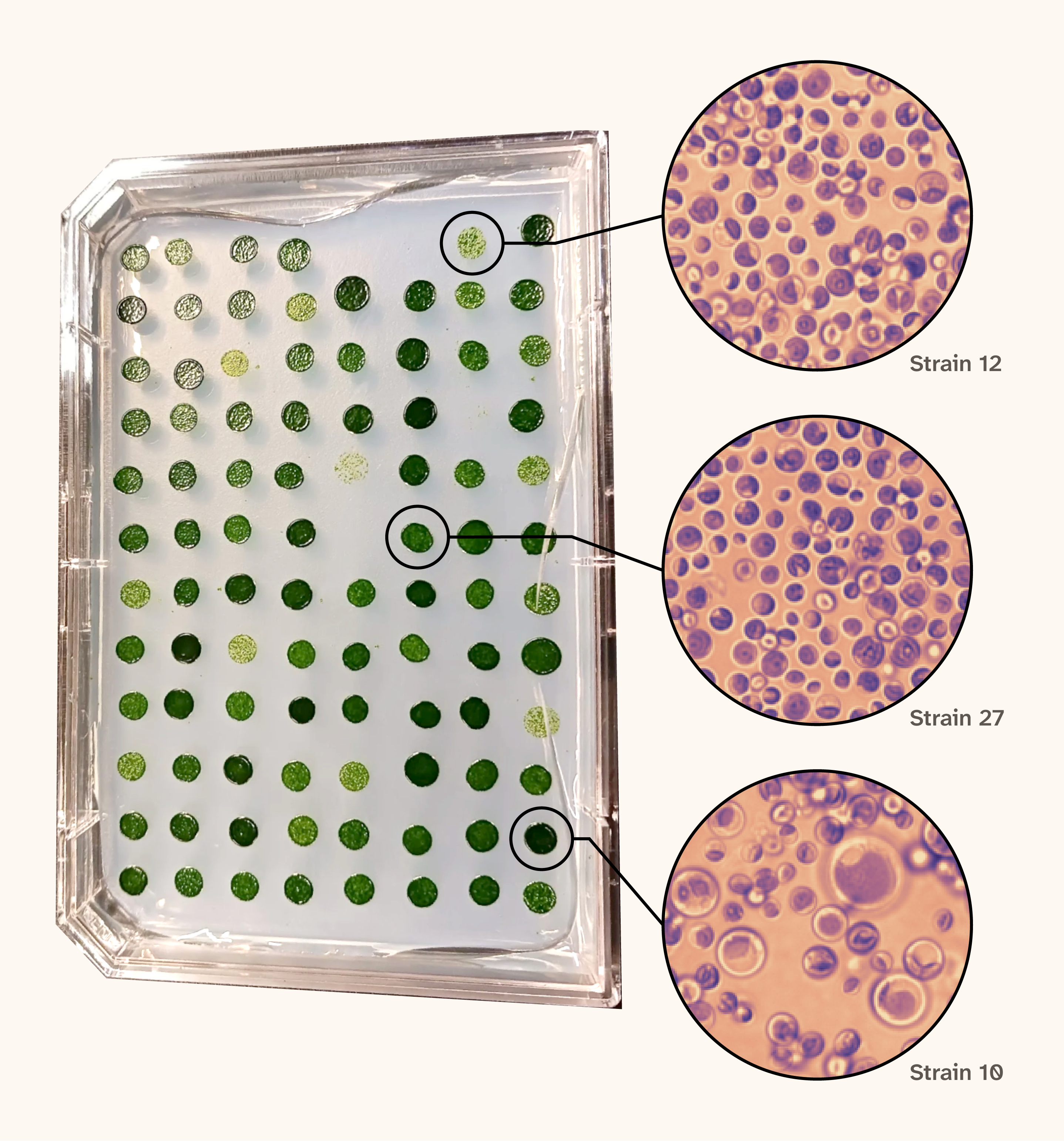
Figure 1. UV mutagenesis produces Chlorella strains with visibly different colonies and cells.
(A) Isolated colonies of UV-mutagenized Chlorella on Tris-acetate-phosphate (TAP) agar plates.
(B–D) Example bright-field images of mutants 12, 27, and 10 grown at 30 °C and imaged in early stationary phase.
Mutant cells were visibly different under the microscope, varying in size, shape, and chlorophyll content. We quantified morphology using our segmentation pipeline, yielding vectors of image-derived features for individual cells from each mutant strain (Table 1). Averaging and normalizing these vectors allowed us to visualize gross differences between mutants at the feature level (Figure 2).
Figure 2. Mutant strains show distinct patterns across image-derived features.
Heatmap showing mean feature values for each mutant strain (rows; n = 91) grown at 22 °C and imaged in early stationary phase, averaged over nine fields of view (more than 100 cells per field). We z-scored each feature (columns) across strains, so 0 is the average strain, and each unit is one standard deviation. We ordered strains by hierarchical clustering (average linkage, Euclidean distance).
To evaluate whether the observed diversity reflected genuine mutagenic effects rather than baseline stochastic variation, we compared phenotypic variability of the mutants with that of wild-type isolates grown and imaged under identical conditions. Mutants were on average farther from the wild-type mean phenotype than wild-type isolates were (p < 0.001, two-sided Mann–Whitney U test; Figure 3), supporting the interpretation that mutagenesis produced phenotypic variation beyond what we see in wild-type isolates.
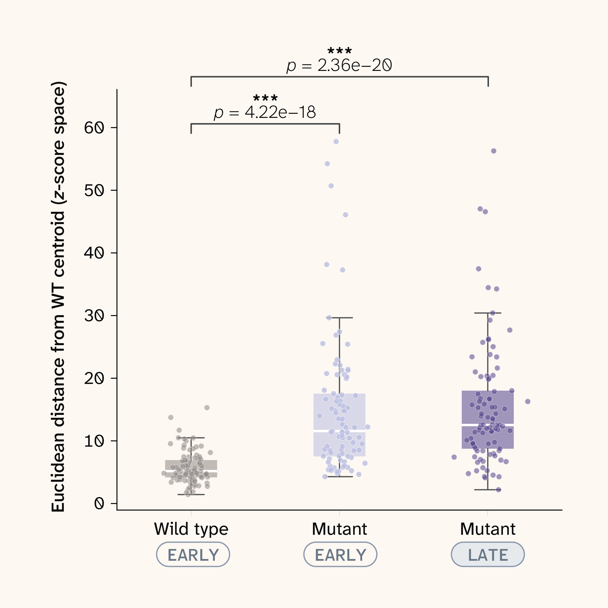
Figure 3. Mutants are more phenotypically diverse than wild-type isolates.
Distance of each strain’s mean phenotype from the wild-type centroid in feature space, z-scored against wild type. We grew wild-type (WT) isolates (n = 96) and mutants (n = 91) at 22 °C and imaged them in early stationary phase; late-stationary mutants are included for context. Each point is one strain. ** denotes p < 0.001. p-values are from two-sided Mann–Whitney U tests of each mutant group against wild type.
Reliable features organize phenotypic variation across conditions
Imaging is a very sensitive phenotypic readout. A single field of view (FoV) captures dozens of morphological features per cell, and small shifts in size, shape, or pigmentation can reveal differences between strains that bulk measurements would miss. That sensitivity may also capture technical artifacts such as image position within a well, local cell density, or small differences in focus and illumination. To interrogate which features reflect real strain-level differences rather than artifacts, we imaged each strain across multiple FoVs per well and treated these images as technical replicates. For each segmented feature in each condition, we calculated an intraclass correlation coefficient (ICC) and then averaged across conditions (Figure 4, A). The ICC is the fraction of a feature's variance that comes from differences between wells rather than from FoV-to-FoV variation. Because each strain occupied a single well per condition, this includes strain differences. A feature with a high ICC separates wells reproducibly, and a feature with a low ICC mostly reflects technical noise.
Most features were highly reliable. Area, perimeter, axis lengths, and convex area had ICCs of 0.91–0.93 in both the bright-field and Cy5 channels, and cell count per FoV was almost perfectly reproducible (ICC = 0.99). Hu moments ranged widely, from 0.31 to 0.82. A small set of features had low ICCs (0.01–0.21): cell orientation and the off-diagonal inertia tensor terms, which depend on orientation. Orientation works as a built-in negative control. Cells settle at random angles, so we didn't expect it to carry any strain-level signal, and it didn't.
Next, we embedded all strains across all conditions into a shared low-dimensional space using t-SNE on z-scored features (Figure 4, B). Conditions occupied distinct but connected regions. Early and late stationary phase separated from each other, and 30 °C pulled away from the cooler temperatures, but there were no sharp boundaries between them. Strains shifted gradually across the embedding rather than falling into discrete clusters.
Figure 4. Features that separate strains reproducibly are the ones that structure the phenotypic landscape.
(A) Intraclass correlation coefficient for each feature, averaged across conditions.
(B–E) t-SNE of z-scored features (one point per field of view) for all strains across all conditions, colored by condition, area (bright-field), Hu moment 0 (bright-field), and orientation (bright-field).
When we colored the embedding by individual features, a feature's reliability tracked how much structure it showed. Area (ICC = 0.93) increased steadily toward one arm of the embedding, where the largest cells were concentrated. Hu moment 0 (ICC = 0.63) showed a patchier pattern, with high values clustered in distinct regions instead of along a single gradient. Orientation (ICC = 0.19) was scattered uniformly, with no spatial organization.
Dimensionality-reduction methods can create apparent structure even from noisy inputs, so the shape of a t-SNE embedding alone isn't strong evidence of a biological signal. The ICC provides a check that doesn't rely on the embedding. Features that reproducibly separate strains are the ones that organize the landscape, and features dominated by technical noise aren't, which is what we’d expect if the embedding reflects reproducible differences between samples rather than an artifact of the method.
The environment observably modulates phenotypes
Before modeling anything, we wanted to answer a basic question: Can our imaging pipeline see biology at all? Temperature and growth phase have large effects on cell state 29–30. They change how fast cells grow, how they divide, and how they use energy. If our pipeline is working, these effects should show up in the images. If they don't, either the cells aren't very responsive to their environment, which would make them a poor system for phenotyping, or our measurements aren't sensitive enough to pick up real changes. We were also interested in the interaction between strain and condition, whether the same environmental change affects different strains in different ways. Before quantifying these interactions, we wanted to see whether they were visible at all.
So, we looked. To make the comparison concrete, we picked three example strains with qualitatively different feature profiles and compared them at three temperatures. Even by eye, temperature changed how the cells looked, and it didn't affect every strain in the same way. Some shifted noticeably in cell size or shape, while others looked much the same from one temperature to the next (Figure 5).
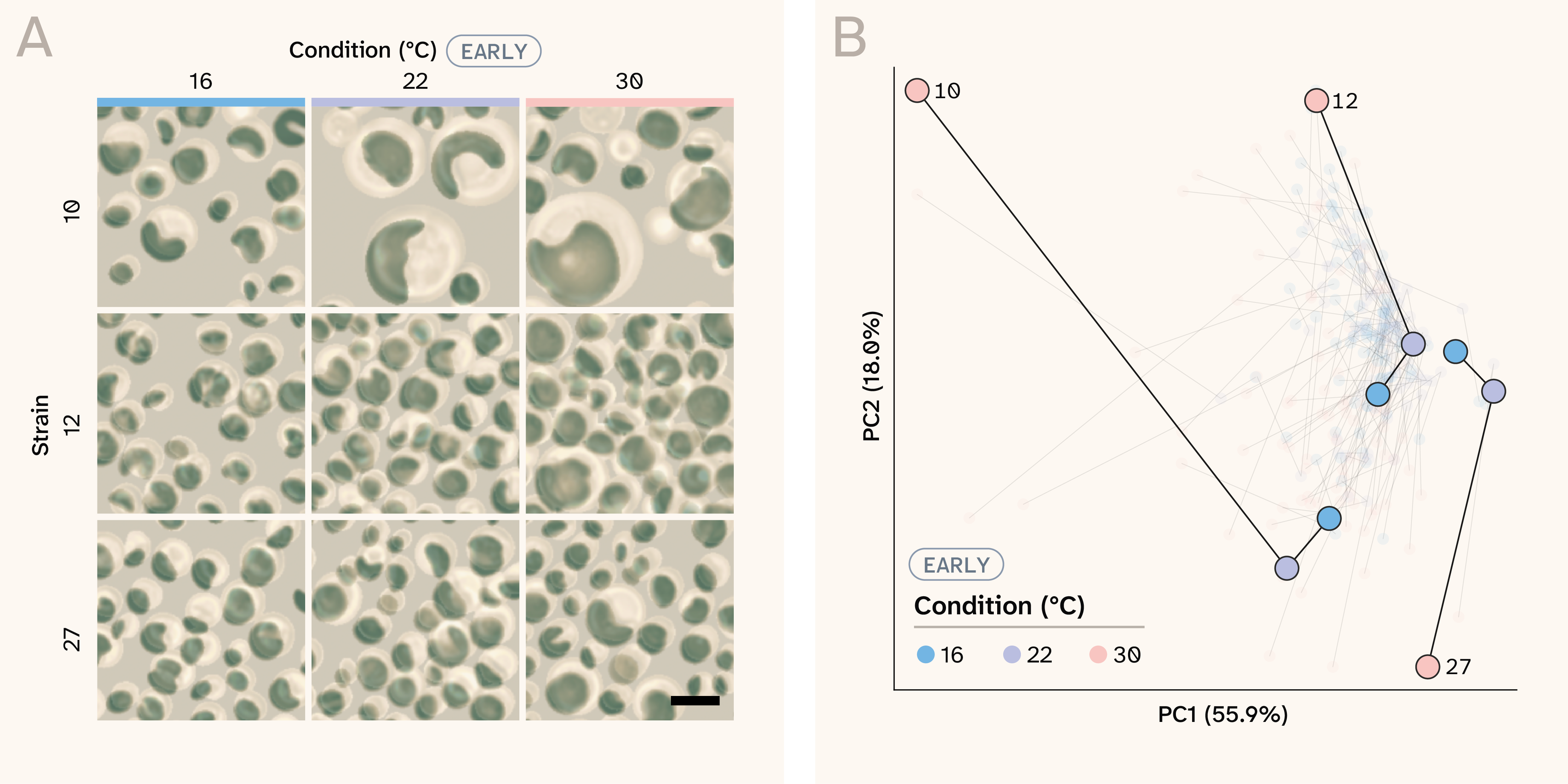
Figure 5. The environment reshapes phenotypes, and strains respond to it differently.
(A) Merged bright-field and Cy5 images of mutants grown at three different temperatures in early stationary phase. Scale bar represents 10 µm.
(B) Trajectories of strains across temperatures in early stationary phase in a principal component analysis (PCA) fit on strain means of the reliable features (mean intraclass correlation coefficient (ICC) of at least 0.5, n = 32) in early stationary phase, z-scored across all temperatures. Principal components 1 and 2 (PC1 and PC2) explain 55.9% and 18.0% of the variance. We highlight example strains 10, 12, and 27, and faint lines show all other strains.
To see whether this held across the whole collection, we projected every strain into a shared principal component space built from the reliable features (mean ICC of at least 0.5, z-scored) and connected each strain's positions across temperatures (Figure 5, B). At 16 °C and 22 °C, strains clustered closely together. At 30 °C, they spread apart, and in different directions: Strain 10 moved far along PC1, strain 12 shifted along PC2, and strain 27 moved the opposite way along PC2. Warmer conditions didn't just shift phenotypes. They exposed differences between strains that were hard to see at cooler temperatures, which could suggest that genetic background shapes how a strain responds to its environment.
This is what we hoped to see. The pipeline detects environmentally driven changes in cell state, and these changes appear to depend on genetic background. But these trajectories are descriptive. A strain that moves far from the rest at 30 °C looks striking, but we don't yet know what a typical trajectory should look like. Some strains might move far simply because of where they start, or because temperature has a large average effect on every strain. To call a strain's response unusual, we need two things. The first is a model that learns how phenotypes generally change across environments, which we build in the next section. The second is a null distribution that indicates how much strain-specific deviation to expect by chance, which we use in the final section to test whether these strain-by-condition interactions are significant.
Phenotypes are predictable in held-out environments
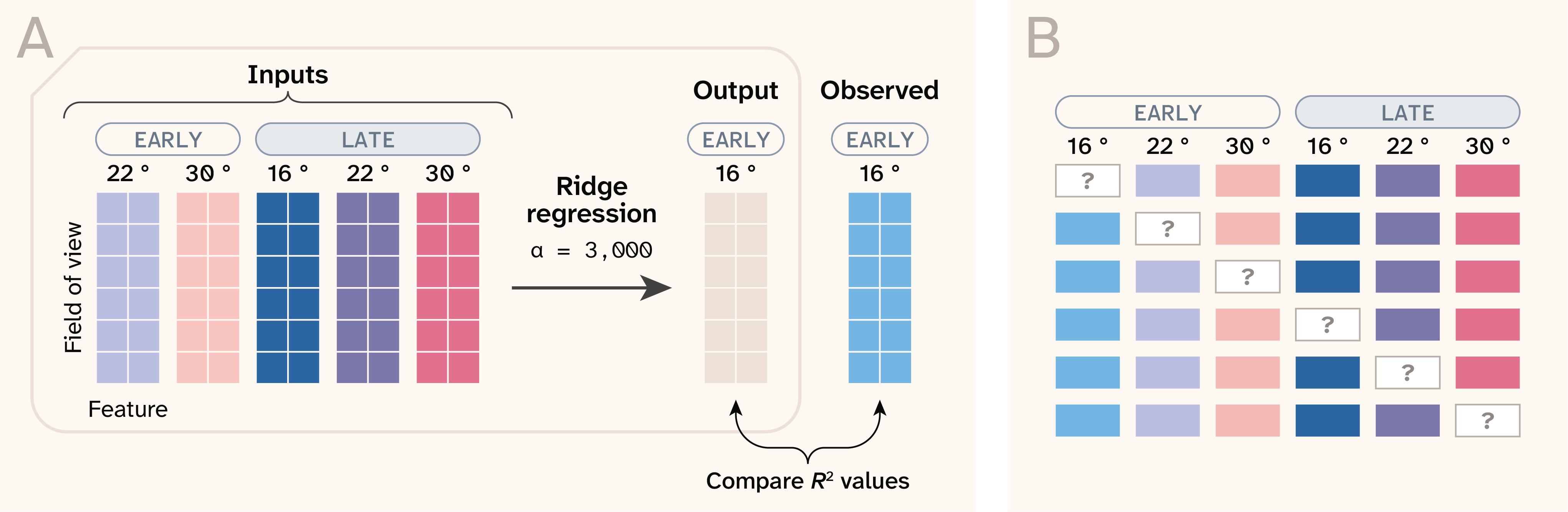
Figure 6. A ridge regression model predicts each strain’s phenotype in a held-out condition.
R2 denotes the coefficient of determination.
The trajectories in the previous section show that phenotypes change across environments, but they don't tell us what change to expect. To build that expectation, we trained a model to learn how phenotypes transform from one environment to another (Figure 6). For each of the six conditions, we held that condition out and trained a ridge regression model (α = 3,000) to predict a strain's features in the held-out condition from its measurements in the other five. We grouped cross-validation folds by well, so the model never saw any field of view from the strain it was predicting. In practice, the model learns from the other strains how phenotypes in five environments map onto the sixth, then applies that mapping to a strain it hasn't seen. We evaluated the model in four ways, each answering a different question.
Figure 7. The model predicts held-out conditions better than an additive baseline.
(A) R2 for each held-out condition from ridge regression and from a recalibrated strain-mean baseline. The baseline uses each strain's mean across the training conditions, mapped onto the held-out condition with a per-feature linear fit. R2 is averaged across all features.
(B) Distance between out-of-fold predicted and observed phenotypes in z-scored feature space, divided by the error of a null model that predicts the population mean for that condition. Each point is one field of view, and the dashed line marks equal performance with the null.
(C) Calibration slopes from regressing observed strain means on predicted strain means. Each point is one feature, and the dashed line marks perfect calibration.
(D) Ridge regression R2 for each feature in each held-out condition.
Does the model learn more than a strain’s average phenotype can tell it? To judge the model, we wanted a strict baseline that already knows the two obvious things: which strain it is and what the environment does to everyone. For each feature, we averaged across the five training conditions for each strain. Using the other strains, we then fit a line mapping those averages onto the held-out condition. This recalibrated strain mean captures how the environment shifts and stretches the entire population, so strains with larger starting values can respond more strongly. What it can’t do is let two strains with the same average respond differently.
Ridge regression beat this baseline in all six held-out conditions, raising R2 by 0.11–0.22 (mean 0.15; Figure 7, A). Averaged across conditions, that's an increase from 0.37 to 0.52. Some of that gain comes from combining information across features, which gives a less noisy estimate of each strain’s phenotype. To separate that from interaction, we also compared the model with a second baseline ridge regression on every feature, but averaged across the training conditions, so it could pool features without seeing how a strain changed from one condition to the next. That baseline reached a mean R2 of 0.43. Pooling features accounts for about 0.06 of the gain, while the remaining 0.09, present in every condition, reflects how each strain behaved in the individual training conditions. The gain was largest at 30 °C in late stationary phase (0.21). Overall R2 ranged from 0.37 at 16 °C early stationary phase to 0.58 at 22 °C late stationary phase. It's an average across all features, including ones we already know are unreliable, so it understates how well the model predicts the reliable features.
How close are the predictions overall? To summarize error across all features at once, we measured the distance between each predicted and observed phenotype in z-scored feature space, for every held-out field of view. We then divided it by the error of a null model that predicts the population mean for that condition (Figure 7, B). A value of 1 means the model is no better than the null. Median ratios ranged from 0.63 at 22 °C in late stationary phase to 0.92 at 30 °C in late stationary phase, so predictions landed about 1.1–1.6 times closer to the observed phenotype than the population mean did. Error was highest at the temperature extremes (30 °C late and 16 °C early stationary phase). We measured these distances for single fields of view, which also vary from field to field within a strain, so part of the remaining error is measurement noise that no model could predict. The wide spread within each condition shows that some measurements are much harder to predict than others.
Are the predictions on the right scale? A model can get the rank order of strains right while compressing all predictions toward the middle, which is a known tendency of ridge regression. To check for this, we regressed observed strain means on predicted strain means for each feature and condition (Figure 7, C). A slope of one means predictions span the same range as reality. Median slopes ranged from about 1.04 to 1.26, so predictions were mildly compressed toward the population mean. That's expected for ridge regression and small enough to correct with a simple linear rescaling, which we apply before testing individual strains in the next section. If predictions were badly compressed, strains with extreme phenotypes would appear to deviate from the model for purely statistical reasons. Slopes far from one came almost entirely from features the model predicted poorly, and 30 °C early stationary phase had the widest spread.
Which features does the model learn? Predictability varied across features and conditions (Figure 7, D). Cell count, which reflects culture density and potentially plate position, was the best-predicted feature in four of six conditions (R2 = 0.68–0.90). The model predicted size features, including area, perimeter, axis lengths, and the inertia tensor eigenvalues, well in both channels. They were more predictable at 22 °C and 30 °C (R2 = 0.70–0.86) than at 16 °C (R2 = 0.40–0.65), which aligns with the lower overall R2 at 16 °C. At the other extreme, orientation and the off-diagonal inertia tensor terms were essentially unpredictable in every condition, as were bright-field Hu moments 1 and 3 in most conditions. These are largely the same features that had low ICCs in our reliability analysis. Orientation, our negative control, behaved exactly as it should. A feature with no reproducible strain-level signal can't be predicted across environments either.
Together, these results show that the model learned real structure in how Chlorella phenotypes respond to the environment. Strain identity and the population-wide environmental effect explain much of it, and the model captures an additional share, part of which may depend on how each strain behaves across conditions. That gives us what the previous section was missing: an expected response for every strain in every environment. In the next section, we ask where that predictability comes from and whether individual strains depart from their expected responses more than chance would allow.
Predictability arises from structured variance
To understand why some phenotypes are more predictable than others, we split each feature's variance into four parts with a two-way factorial ANOVA: strain, environment, their interaction, and residual (Figure 8, A). With nine fields of view per well, the residual is field-to-field variation within one strain in one condition. That separates measurement noise from the other terms. Because we grew each strain in a single well per condition, the interaction term also includes any culture-to-culture variation specific to that well, so it’s an upper bound on true strain-by-environment interaction.
How variance was distributed varied a lot across features. For cell count and the size features in both channels, such as area, perimeter, and axis lengths, strain was the largest component, and residual variance was small. Pixel intensity was dominated by the condition instead. For orientation, the off-diagonal inertia tensor terms, and most bright-field Hu moments, residual variance made up most of the total. These are the same features that failed our reliability analysis.
Figure 8. Features with more strain-level variance and less noise are more predictable.
(A) Heatmap of partitioned variance per feature.
(B) Bar chart showing Pearson correlations between ridge R2 values and fractional variances.
(C) Scatter plot of correlation between mean per-feature ridge R2 value and the fractional residual variance of each feature.
As expected, this variance structure largely explains how well the model performed. Across features, mean ridge R2 was strongly correlated with the fraction of variance from strain (Pearson's r = 0.88) and strongly anticorrelated with the residual fraction (r = −0.96) (Figure 8, B). It was moderately correlated with the interaction (r = 0.61) and environment (r = 0.42) fractions. Because the four fractions sum to 1, these correlations aren’t independent of each other. Features with a residual fraction below about 0.2 all had a mean R2 of at least 0.4, while most features with a residual fraction above 0.6 were essentially unpredictable (Figure 8, C). The correlation with strain variance is partly built into the design. When the model predicts a held-out condition from the others, it relies on strain-level signals that persist across conditions, so features dominated by strain effects will tend to be more predictable by construction. The result is still useful in practice. A feature's residual fraction sets a ceiling on how predictable it can be, and it tells us in advance which features are worth modeling.
The interaction component is where this becomes interesting. For most reliable features, the strain-by-environment interaction accounted for about 0.1–0.3 of the variance, roughly as much as the environment itself. Ridge regression also beats a baseline that pools every feature but can’t see condition-specific responses, in every condition. That’s consistent with the model capturing part of that interaction, though the gain could also come from weighting more reliable conditions more heavily or from well-specific effects. How a strain responds to temperature isn't arbitrary. To a meaningful degree, we can predict it from how that strain behaves in other conditions. That's what lets us return to the question we could only describe earlier: When a strain changes across environments, is that change surprising?
Strains 37 and 94 make a good test case (Figure 9, A). We chose them because their difference in cell count changed more across temperatures than that of any other pair in the collection. In late stationary phase, they look similar at 16 °C. By 30 °C, strain 94 has changed dramatically: far fewer cells per field of view, and the cells that remain are large and round. Strain 37 changes much less. Without a model, we'd have no way of knowing whether strain 94's response is unusual or just an extreme version of what the collection does. With the model, we can compare each strain's observed reaction norm with the one predicted from its other conditions 31.
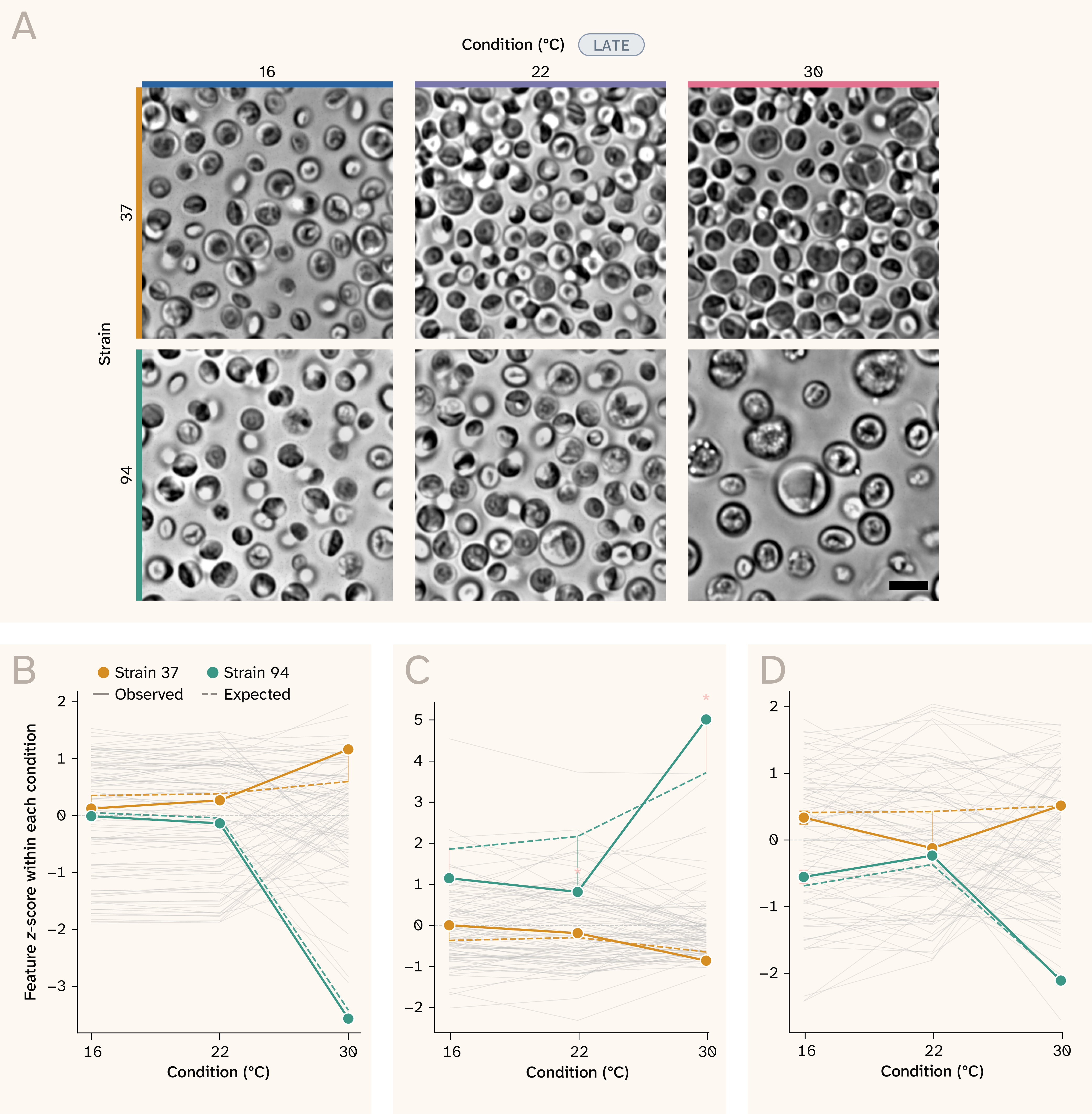
Figure 9. The model separates expected phenotypic responses from unexpected departures.
(A) Pair of mutants (37 and 94) grown at different temperatures and imaged in the late stationary phase. Scale bar represents 10 µm.
(B–D) Observed (solid) and expected (dashed) reaction norms for cell count (B), area (C), and eccentricity (D), z-scored across strains within each condition. Error bars are ± 1 standard error of the mean (SEM) across fields of view, gray lines show all other strains, and an asterisk marks a departure that passes Benjamini–Hochberg correction (q < 0.05).
For cell count and eccentricity, strain 94's response was almost entirely expected (Figure 9, B, D). At 30 °C, its count fell to −3.57 standard deviations (SD) against an expected −3.42 SD, and its eccentricity landed at −2.11 SD against an expected −2.09 SD. Strain 37 didn't depart significantly from its predicted reaction norm in any of the three features. Area was different. The model expected strain 94's cells to grow steadily larger than those of other strains as temperature increased (Figure 9, C). Instead, they stayed roughly close to the same from 16 °C to 22 °C (observed = 0.82 SD, expected = 2.17 SD; q = 0.001), then overshot the prediction at 30 °C (observed = 5.01 SD, expected = 3.72 SD; q = 0.004). Because we grew each strain in a single well per condition, confirming that this reflects strain 94 rather than that particular culture would require replicate wells. These were the only departures among these strains, features, and conditions that passed false discovery rate (FDR) correction, though p-values assume residuals are normal across strains. Most of strain 94's dramatic phenotype at 30 °C is a predictable consequence of how it behaves elsewhere. What isn't predictable is the shape of its area response: flat through 22 °C, then a sharp jump.
This is the step up from observing phenotypic responses to evaluating them. When we first looked at strains across environments, we could only see that they responded differently. Now we can say what response to expect for each strain, how far its actual response departs from that expectation, and whether the departure is larger than typical. Among the strains and features we examined, most responses were predictable. In a screen of targeted knockouts, a strain whose response the model can't explain is exactly the kind of result we'd want to catch.
Key takeaways
Chlorella is ready for its next step. Label-free imaging captured phenotypic diversity among mutagenized strains, and most features meaningfully contributed to separation of strains across fields of view. Those differences shift with temperature and growth stage, and they shift in ways a model can learn. Using measurements from five conditions, our model predicted strains’ phenotypes in a sixth better than baselines built from each strain’s average phenotype (mean R2 of 0.52 vs. 0.37), and most of that advantage held up against a baseline that pools all features (0.43). That gives us a starting point for a screen: readouts that reliably separate strains, and an expected response for each strain that future knockouts can be compared against.
The broader lesson is about how to take on a new organism. It’s tempting to go straight from “this organism looks interesting” to building genetic tools and launching a screen, but a de-risking analysis such as this tells you which measurements to trust, how strongly the organism responds to perturbation, and whether those responses are consistent enough to interpret. None of that is specific to Chlorella. As we and others look across the tree of life for new experimental systems, a tractability check like this is a cheap way to find out whether an organism is worth the deeper investment.
A few lessons from this analysis that may be useful beyond Chlorella:
- Dramatic isn’t the same as surprising. Strain 94 changed dramatically at 30 °C, but most of that change was predictable from how the strain behaved in other conditions. Without an expected response for each strain, the most eye-catching hits in a screen can be the least informative.
- Measure your noise before your biology. Imaging several fields of view per well costs almost nothing extra, and it lets us score every feature’s reliability before any modeling. Those measurements then helped predict which features the model could learn.
- Changing conditions can expose hidden variation. Several strains looked alike at 16 °C and 22 °C and only spread apart at 30 °C. When choosing screening conditions, it’s worth looking for ones that pull strains apart, not just the standard growth conditions.
- Replicate wherever you want to make claims. We grew each strain in a single well per condition, with one plate per temperature. That was enough to show the system is tractable, but it means we can’t fully separate a strain’s response from that particular culture or plate. If you plan to call individual strains as hits, build replicate wells and plates into the design from the start.
Next steps
This analysis tells us Chlorella is worth pursuing. Here’s where we’d take it next.
The most immediate step is building the genetic tools to perturb Chlorella directly. Gene editing in C. vulgaris is much less established than in model algae like Chlamydomonas reinhardtii 32–33, and we’re currently working to change that. With those tools in hand, we plan to apply this phenotyping framework to knockouts of genes identified as Zoogle hits. If Chlorella is to serve as a perturbation platform, the critical test is whether losing a functionally conserved gene produces a phenotypic shift that’s detectable, interpretable, and distinct from the variation we see across wild-type and mutagenized backgrounds. From there, we can return to the question that brought us to Chlorella in the first place. By rescuing knockouts with their human orthologs and testing human disease variants, we hope to use it as a system for studying human biology.
We also plan to expand the environmental conditions we survey. Strains that looked alike at 16 °C and 22 °C only spread apart at 30 °C, which suggests that other conditions may expose differences we haven’t seen yet. Temperature and growth stage were enough to establish proof of concept, but they cover only a narrow slice of the possible perturbation space. A broader sweep, including additional stressors, nutrient conditions, and light regimes, would give a richer picture of how Chlorella responds to its environment and help clarify which features are broadly informative and which are condition-specific.
We’re also exploring phenotyping modalities beyond imaging. Most of the strain-level signal we found came from cell size and shape, which tells us how cells look but not what they’re made of. Raman spectroscopy offers a label-free window into cellular composition and has been used to track metabolic and stress states in algae 34–36. Pairing it with imaging could reveal phenotypes that morphology alone would miss.
As we’re building Chlorella’s genetic toolkit now, we’d especially love to hear from others working on related problems. If you’ve developed transformation or gene-editing methods for Chlorella or other green algae, please reach out or leave a comment. Additionally and more broadly, if you’ve run similar tractability checks in other non-model organisms or see a better way to score phenotypic readouts, we’d love to hear it.
Be the first to comment on this publication.